| *featured, #machine-learning, #python, #series__perceptron | |||
19-line Line-by-line Python Perceptron |
|||
"""
MIT License

Copyright (c) 2018 Thomas Countz

Permission is hereby granted, free of charge, to any person obtaining a copy
of this software and associated documentation files (the "Software"), to deal
in the Software without restriction, including without limitation the rights
to use, copy, modify, merge, publish, distribute, sublicense, and/or sell
copies of the Software, and to permit persons to whom the Software is
furnished to do so, subject to the following conditions:

The above copyright notice and this permission notice shall be included in all
copies or substantial portions of the Software.

THE SOFTWARE IS PROVIDED "AS IS", WITHOUT WARRANTY OF ANY KIND, EXPRESS OR
IMPLIED, INCLUDING BUT NOT LIMITED TO THE WARRANTIES OF MERCHANTABILITY,
FITNESS FOR A PARTICULAR PURPOSE AND NONINFRINGEMENT. IN NO EVENT SHALL THE
AUTHORS OR COPYRIGHT HOLDERS BE LIABLE FOR ANY CLAIM, DAMAGES OR OTHER
LIABILITY, WHETHER IN AN ACTION OF CONTRACT, TORT OR OTHERWISE, ARISING FROM,
OUT OF OR IN CONNECTION WITH THE SOFTWARE OR THE USE OR OTHER DEALINGS IN THE
SOFTWARE.
"""

import numpy as np

class Perceptron(object):

    def __init__(self, no_of_inputs, threshold=100, learning_rate=0.01):
        self.threshold = threshold
        self.learning_rate = learning_rate
        self.weights = np.zeros(no_of_inputs + 1)

    def predict(self, inputs):
        summation = np.dot(inputs, self.weights[1:]) + self.weights[0]
        if summation > 0:
          activation = 1
        else:
          activation = 0
        return activation

    def train(self, training_inputs, labels):
        for _ in range(self.threshold):
            for inputs, label in zip(training_inputs, labels):
                prediction = self.predict(inputs)
                self.weights[1:] += self.learning_rate * (label - prediction) * inputs
                self.weights[0] += self.learning_rate * (label - prediction)
Get the code: here, “regression” type tests here.
So far, we’ve been doing a lot of learning, with not a lot of “machine.” Today, that changes, because we’re going to implement a perceptron in Python.
What makes this Python perceptron unique, is that we’re going to be as explicit as possible with our variable names and formulas, and we’ll go through it all, line-by-line, before we get clever, import a bunch of libraries, and refactor.
Before we begin, we’ll start with a little recap and summary.
Recap & Summary
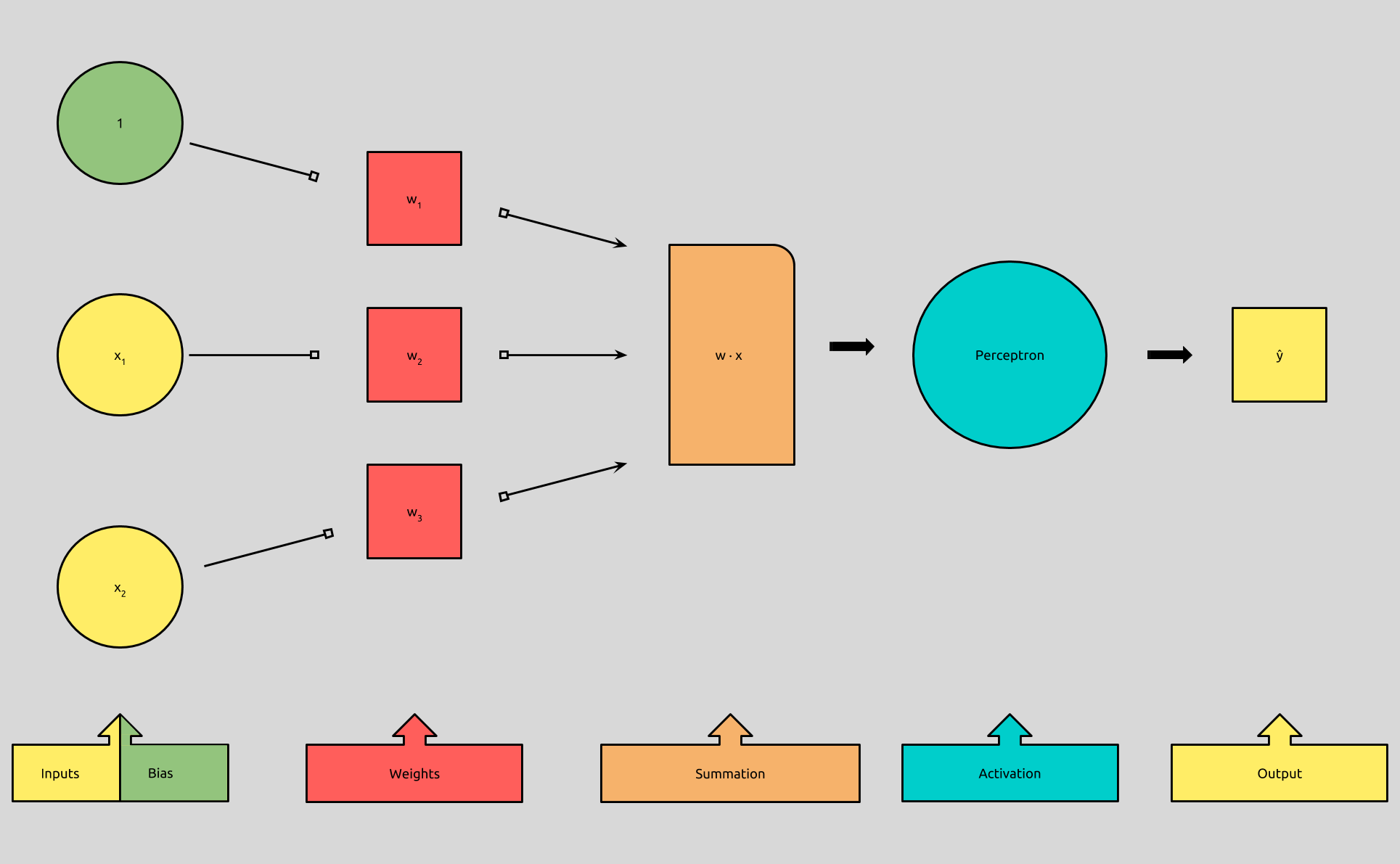
In Perceptron in Neural Networks, we looked at what a perceptron was, and we discussed the formula that describes the process it uses to binarily classify inputs. We learned that the perceptron takes in an input vector, x, multiplies it by a corresponding weight vector w, and then adds it to a bias, b. It then uses an activation function, (the step function, in this case), to determine if our resulting summation is greater than 0, in order to classify it as 1 or 0.
](/assets/images/perceptron-equation-simple.png)
In Perceptron Implementing AND - Part 1, we looked at how we could use a perceptron to mimic the behavior of an AND logic gate. We walked through, and reasoned about, how to determine the values of the weight vector, w, and the bias, b, in order for our perceptron to accurately classify the inputs from the AND truth table.
In Perceptron Implementing AND - Part 2, we looked at the Perceptron Learning Rule. We learned that by using labeled data, we could have our perceptron predict an output, determine if it was correct or not, and then adjust the weights and bias accordingly. In the end, we ended up with two formulas to describe the perceptron:
f(x) = 1 if w · x + b > 0
       0 otherwise

w <- w + (y - f(x)) * x
In Summary, we now have in our arsenal a classification algorithm.
Classification is a subcategory of supervised learning where the goal is to predict the categorical class labels of new instances, based on past observations.
- Sebastian Raschka, Vahid Mirjalili, Python Machine Learning — 2nd Ed.
Supervised learning, is a subcategory of Machine Learning, where learning data is labeled, meaning that for each of the examples used to train the perceptron, the output in known in advance.
When considering what kinds of problems a perceptron is useful for, we can determine that it’s good for tasks where we want to predict if an input belongs in one of two categories, based on its features and the features of inputs that are known to belong to one of those two categories.
These tasks are called binary classification tasks. Real-world examples include email spam filtering, search result indexing, medical evaluations, financial predictions, and, well, almost anything that is “binarily classifiable.”
Today, we’ll be continuing with AND:
 A   B  | AND
--- --- |-----
 1   1  |  1
 1   0  |  0
 0   1  |  0
 0   0  |  0
The Code:
I would be remiss to say, “that’s it,” because it took me quite a bit of work to write these 19 lines (minus newlines), but when considering what these 19 lines can do, it’s kind of surprising that this is all it takes. Let’s walk through it.
Line-by-line
import numpy as np
If you’re like me, not familiar with the numpy module, the only important thing to know here is that we’re using it to evaluate our dot product w · x during our summation. numpy lets us create vectors, and gives us both linear algebra functions and python list-like methods to use with it. We access its functions by calling them on np.
class Perceptron(object):
Here, we’re creating a new class Perceptron. This will, among other things, allow us to maintain state in order to use our perceptron after it has learned and assigned values to its weights.
def __init__(self, no_of_inputs, threshold=100, learning_rate=0.01):
In our constructor, we accept a few parameters that represent concepts that we looked at the end of Perceptron Implementing AND - Part 2.
The no_of_inputs is used to determine how many weights we need to learn.
The threshold, is the number of epochs we’ll allow our learning algorithm to iterate through before ending, and it’s defaulted to 100.
The learning_rate is used to determine the magnitude of change for our weights during each step through our training data, and is defaulted to 0.01.
The threshold and learning_rate variables can be played with to alter the efficiency of our perceptron learning rule, because of that, I’ve decided to make them optional parameters, so that they can be experimented with at runtime.
self.threshold = threshold
self.learning_rate = learning_rate
These two lines set the threshold and learning_rate arguments to instance variables.
self.weights = np.zeros(no_of_inputs + 1)
Here, we initialize our weight vector. np.zeros(n), will create a vector with an n-number of 0’s. Here, we use the no_of_inputs, (which again, is number of inputs in our input vector, x), plus 1.
Remember in Perceptron Implementing AND - Part 2, we move our bias into the weight vector, so that we didn’t have to deal with it independently of our other weights? This bias is the +1 to our weight vector, and is referred to as the bias weight.
def predict(self, inputs):
Now, we define our predict method. This is the method we first looked at, way back in Perceptron in Neural Networks. This method will house the f(x) = 1 if w · x + b > 0 : 0 otherwise algorithm.
The predict method takes one argument, inputs, which it expects to be an numpy array/vector of a dimension equal to the no_of_inputs parameter that the perceptron was initialized with on line 5.
summation = np.dot(inputs, self.weights[1:]) + self.weights[0]
This is where the numpy dot product function comes in, and it works exactly how you might expect. np.dot(a, b) == a · b. It’s important to remember that dot products only work if both vectors are of equal dimension. [1, 2, 3] · [1, 2, 3, 4] is invalid. Things get a bit tricky here because we’ve added an extra dimension to our self.weights vector to act as the bias.
There are two options here, either we can add a 1 to the beginning of our inputs vector, like we discussed in Perceptron Implementing AND - Part 2, or, we can take the dot product of the inputs and the self.weights vector with the the first value “removed”, and then add the first value of the self.weights vector to the dot product. Either way works, I just happened to think that this way was cleaner.
We then store the result in the variable, summation.
if summation > 0:
  activiation = 1
else:
  activation = 0
return activation
This is our step function. It kind of reads like pseudocode: if the summation from above is greater than 0, we store 1 in the variable activation, otherwise, activation = 0, then we return that value.
We don’t need the temporary variable activation, but for now, the goal is to be explicit.
def train(self, training_inputs, labels):
Next, we define the train method, which takes two arguments: training_inputs and labels.
training_inputs is expected to be a list made up of numpy vectors to be used as inputs by the predict method.
labels is expected to be a numpy array of expected output values for each of the corresponding inputs in the training_inputs list.
In essence, the input vector at training_inputs[n] has the expected output at labels[n], therefore len(training_inputs) == len(labels).
for _ in range(self.threshold):
This creates a loop wherein the following code block will be run a number of times equal to the threshold argument we passed into the Perceptron constructor. If one hasn’t been passed in, it’s defaulted to 100 epochs. Because we don’t care to use an iterator variable, convention has us set it to _.
for inputs, label in zip(training_inputs, labels):
There are three important steps happening in this line:
-
We
ziptraining_inputsandlabelstogether to create a newiterableobject -
We loop through the new object
-
While we iterate through, we store each elements in the
training_inputslist into theinputsvariable, and each of the elements inlabels, in the variablelabel.
In the code block after this line, when we reference label, we get the expected output of the input vector stored in the inputs variable, and we do this once for every inputs/label pair.
prediction = self.predict(inputs)
Here, we pass the inputs vector into our previously defined predict method, and we store the result in the prediction variable.
self.weights[1:] += self.learning_rate * (label - prediction) * inputs
This is almost all of the learning rule implementation:
w <- w + α(y — f(x))x
We find the error, label — prediction, then we multiply it by our self.learning_rate, and by our inputs vector, we then add that result to the weight vector (with the bias weight removed), and store it back into self.weights[1:].
Remember that self.weights[0] is our bias weight, so we can’t add self.weights and inputs vectors directly, as they’re of different dimensions.
There were several options to take care of this, but I think the most explicit was is to mimic what we have done early, by only considering the vector created by “removing” the bias weight at self.weights[0].
We can’t just ignore the bias, so we deal with it next:
self.weights[0] += self.learning_rate * (label - prediction)
We update the bias in the same way as the other weights, except, we don’t multiply it by the inputs vector.
TA DA!
In just 19 lines of explicit code, we were able to implement a perceptron in Python!
Usage
Let’s put it to work and finally wrap up implementing AND
import numpy as np
from perceptron import Perceptron
First, we import numpy so that we can create our vectors, then we import our new perceptron.
training_inputs = []
training_inputs.append(np.array([1, 1]))
training_inputs.append(np.array([1, 0]))
training_inputs.append(np.array([0, 1]))
training_inputs.append(np.array([0, 0]))
Next, we generate our training data. These inputs are the A and B columns from the AND truth table stored in an array of numpy arrays, called training_inputs.
labels = np.array([1, 0, 0, 0])
Here, we store the expected outputs, or labels in the label variable, making sure that each label index lines up with the index of the input it’s meant to represent.
perceptron = Perceptron(2)
We instantiate a new perceptron, only passing in the argument 2 therefore allowing for the default threshold=100 and learning_rate=0.01. Note that such a large threshold and such a small learning rate probably isn’t needed, so feel free to play around to find what’s most efficient! What happens if learning_rate=10? What if threshold=2?
perceptron.train(training_inputs, labels)
Now we train the perceptron by calling perceptron.train and passing in our training_inputs and labels.
This should finish rather quickly. Even though there are 100 epochs, our training data is so small and numpy is very efficient!
inputs = np.array([1, 1])
perceptron.predict(inputs)
#=> 1

inputs = np.array([0, 1])
perceptron.predict(inputs)
#=> 0
That’s it! Now, we can start to use the perceptron as a logic AND!
It may seem a bit bizarre that we’ve trained our perceptron with four inputs and we only really need it to classify those four inputs. Is that all perceptrons are good for? No! Remember, perceptrons can be used to classify almost any number of binarily classifiable things, (though there are some major caveats, see below).
What would happen if you removed one of the training inputs? Removed two of them? Are you able to remove the [1, 1] training input? What other logic operators can you train the perceptron on? What happens if we add more inputs?
Test! Experiment! Play!
Conclusion
This concludes our AND implementation, so now is a good time to sum up everything we’ve learned.
Perceptrons were first published in 1957 by Frank Rosenblatt at the Cornell Aeronautical Laboratory. He proposed a rule that could automatically determine the weights **for each of the artificial neuron’s **input features, (one input vector example), by using supervised learning to determine a decision boundary, (see below), between two binary classes.
The perceptron classifies inputs by finding the dot product of an input feature vector and weight vector and passing that number into a step function, which will return 1 for numbers greater than 0, or 0 otherwise.
f(x) = 1 if w · x + b > 0
       0 otherwise
In order to determine the weights, the Perceptron Learning Rule:
-
Predicts an output based on the current weights and inputs
-
Compares it to the expected output, or label
-
Update its weights, if the prediction **!= the **label
-
Iterate until the epoch threshold has been reached
To update the weights during each iteration, it:
-
Finds the error by subtracting the prediction from the label
-
Multiplies the error and the learning rate
-
Multiplies the result to the inputs
-
Adds the resulting vector to the **weight **vector
w <- w + α(y - f(x))x
Appendix and Further Exploration
There are a few concepts we haven’t touched on yet. Notably, the limitations of the perceptron.
The Perceptron Convergence Theorem is, from what I understand, a lot of math that proves that a perceptron, given enough time, will always be able to find a decision boundary between two linearly separable classes.
It is important to note that the convergence of the perceptron is only guaranteed if the two classes are linearly separable and the learning rate is sufficiently small. If the two classes can’t be separated by a linear decision boundary, we can set a maximum number of passes over the training dataset (epochs) and/or a threshold for the number of tolerated misclassifications — the perceptron would never stop updating the weights otherwise.
- Sebastian Raschka, Vahid Mirjalili, Python Machine Learning — 2nd Ed.
Linearly separable means that there exists a linear hyperplane, (line), that can separate input vectors into their correct classes; one class’ vectors falling on one side of the hyperplane, and the other class’, on the other.
In terms of our binary operator AND, linear separability means that:
If…
We plot each of our
*A*and*B*inputs, from our truth table, as points,*(A, B)*, on a 2-D plane…
Then..
We could draw a single line on that plane in such a way so that all of the
*(A, B)*points on one side of the line are the*A*and*B*inputs that give us*1*, and all the points on the other side, give us*0*.
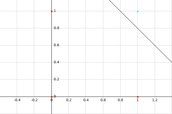
Here is ourAND and its truth table:
( A , B ) | AND
---  ---  |-----
( 0 , 0 ) |  0
( 0 , 1 ) |  0
( 1 , 0 ) |  0
( 1 , 1 ) |  1
We see that all of the pairs of inputs that return 0 are red and on one side of the line, and the input that gives us 1, is on the other side of the line.
This is a graphical representation of what our perceptron does! Our perceptron defines a line to draw in the sand, so to speak, that classifies our inputs binarily, depending on which side of the line they fall on! This line is call the decision boundary*, and when employing a single perceptron, we only get one.*
In other words, if there is no single line that can separate our training data into two classes, our perceptron will never find weights that can satisfy all of our data. It doesn’t take long to hit this limitation. Take a look the XOR Perceptron Problem.
Perceptrons have gotten us pretty far, but we’re not done with them yet. Now that we’ve gotten our hands on some code, we can begin digging deeper into using Python as a tool to further explore machine learning and neural networks.
Next, we’ll refactor our perceptron code, take a look at how we can use our model to classify more complex data, and look at how to use tools like matplotlib to visualize decision boundaries.
Resources
- Perceptron Convergence Theorem
- Python Machine Learning — 2nd Ed. by Sebastian Raschka & Vahid Mirjalili
- Single-Layer Neural Networks and Gradient Descent
- 10.2: Neural Networks: Perceptron Part 1 — The Nature of Code
- Appendix F — Introduction to NumPy from Introduction to Artificial Neural Networks and Deep Learning A Practical Guide with Applications in Python by Sebastian Raschka