| #machine-learning, #python, #series__perceptron | |||
Automating Perceptron Learning AlgorithmLearning Machine Learning Journal #2 |
|||
In Perceptron Implementing AND, Part 1, we looked at implementing the behavior of AND with a perceptron. We set up our perceptron with its inputs and expected outputs, and we sort of reasoned about what our weights and bias should be, in order to get the output we wanted.
Even for just a single artificial neuron, with only two binary inputs, a single binary output, and a complete set of training data, that was still a considerable amount of work, which resulted in mimicking behavior of a simple logic statement.
If we consider that neural networks are made up of dozens, thousands, or even 160 billion neurons, we can see that manually tuning our weights and biases is simply out of the question.
When we talk about a neural network “learning,” or “training,” this tuning process is exactly what we’re talking about. Our networks can learn to assign its own weights and biases, based on a set of training data, where the inputs and expected outputs are known.
Our neuron does this by iterating through training data, and updating the weights and bias after each set of inputs. Once our neuron determines that it has found parameters that successfully classify all of the training data, the learning process is complete, and the weights and biases can then be used to classify data that wasn’t in the training set!
Seeing that our AND truth table is a type of training data, and we have our model of a network, (even if it’s only one neuron), we can implement this learning behavior, and that’s what we’ll take a look at today.
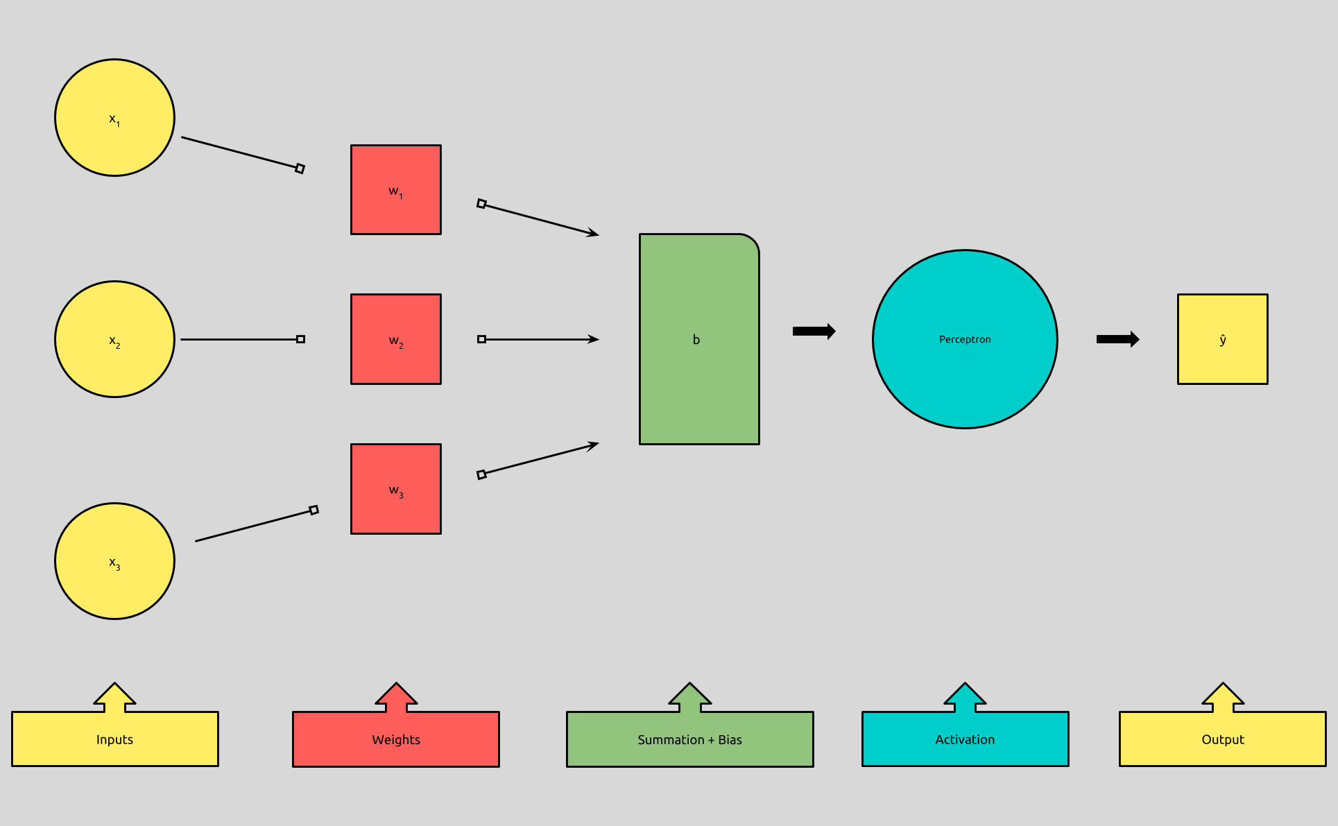
A Bias is the Weight of an Always-Active Input
Before we take a look at the learning process, we’re going to tweak our perceptron model, just a little bit:
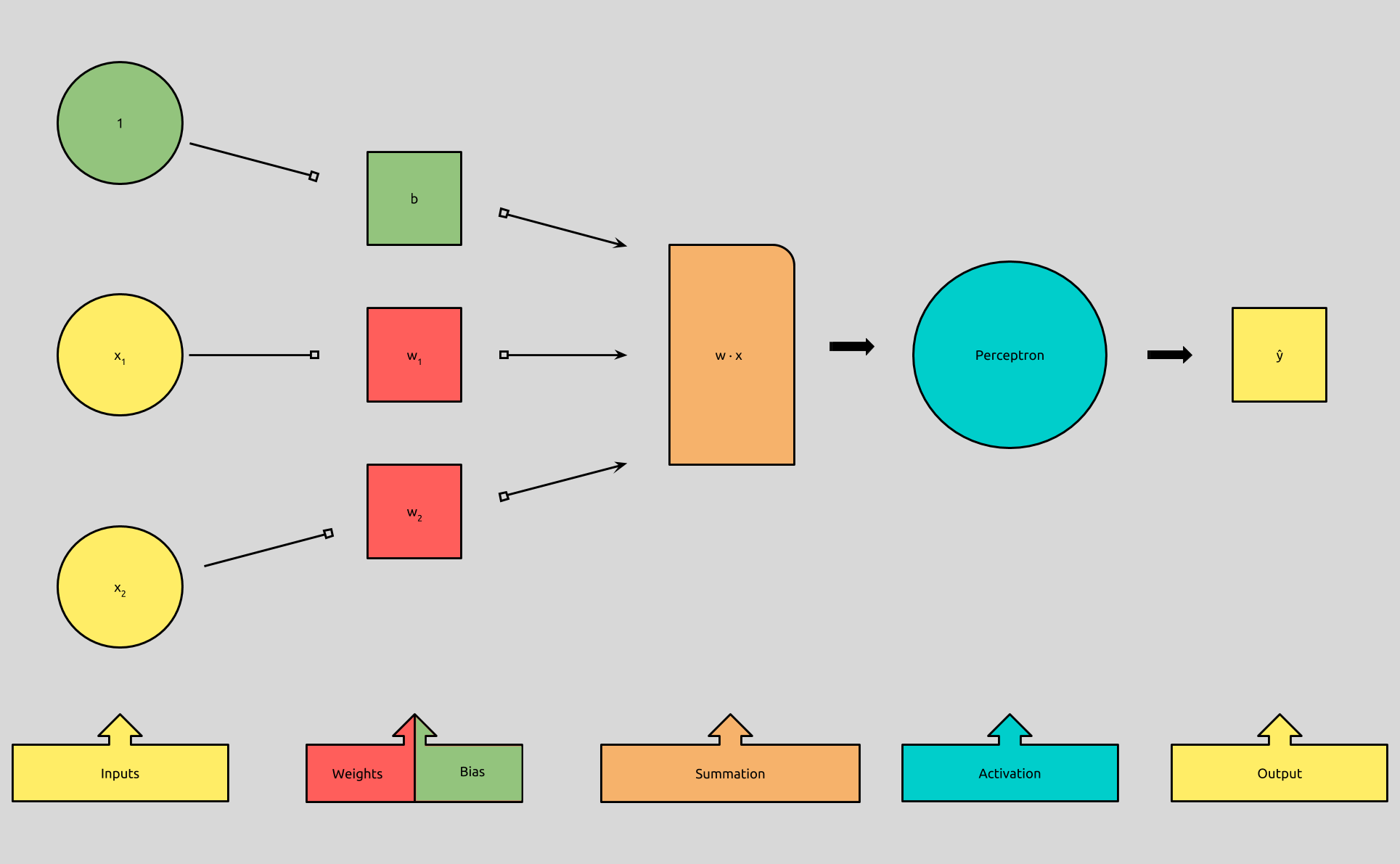
It turns out that the algorithm that determines the weights for each input, is the same algorithm that determines the bias. Because of this, it’s more efficient to lump the concept of a bias in with the other inputs by adding an additional input with an activation of 1, and allow our algorithm to treat the weight of that new input, as the bias.
](/assets/images/perceptron-equation-simple.png)
If you remember our perceptron formula, (pictured to the left), you’ll recall that we add the dot product of vectors w and x, to the bias, b, to get what is called the weighted sum. Expanded, it looks like this:
(w1 * x1) + (w2 * x2) + ... + (wn * xn) + b
Where wn is the weight of input xn.
We add the product of all n-numbered w’s and their n-numbered x’s together, and then we add that result to the bias, b.
In this equation, we can also represent b, by adding another input whose activation is always 1, and multiplying it by a weight equal to b.
(w1 * x1) + (w2 * x2) + ... + (wn * xn) + (b * 1)
You’ll even sometimes see b as (w0 * x0), where x0 = 1.
Our inputs x ... xn will never be changed by our learning algorithm, and therefore, neither will our new input,1. Our algorithm now can focus only on adjusting the weights, which now also include our bias.
We can think of this new perceptron algorithm like this:
f(x) = 1 if w · x > 0
       0 otherwise
As long as we explicitly add an input with an activation of 1, and a weight equal to b.
How Perceptrons Learn
These are the abstract steps that our perceptron will take in order to learn, i.e., converge on a set of values for its weights that will accurately classify all of our training input:
-
Initialize the weights, sometimes randomly, or more simply, establish them all to
0. -
For each set of inputs in the set of training examples our perceptron will:
-
Predict an output
-
Compare it to the expected output
-
Update its weights, if the expected output != the actual output.
-
Move to next set of inputs.
There are a few new concepts we’ll want to define.
First, we’ll need to know how well our perceptron is doing.
Given that our neuron produces an output, and we know what we expect the output to be, we can define how well our neuron is doing like this:
expected_output - actual_output
Which we’ll notate like this:
e = y - f(x)
Where e, for error, is equal to our expected output y, minus the output of our perceptron function, f, given inputs x.
Given that y and f(x) are binary, y — f(x), will produce only one of three values, given any x:
y   f(x) | y - f(x)
---  ---  | --------
 1    1   |    0
 0    0   |    0
 1    0   |   -1
 0    1   |    1
Next, we’ll see how we can use this information to adjust our weights.
The goal: get y — f(x) closer to 0.
The intuition behind this learning algorithm, developed by Frank Rosenblatt, who you’ll remember as the creator of the perceptron, follows a simple rule:
If the neuron activates, when we want it not, suppress it.
If the neuron does not activate, when we want it so, excite it.
If the neuron performs as asked, do nothing.
—Frank Rosenblatt
We know how to check how well our neuron is doing, so now, we’ll need to establish how we can excite it, suppress it, or do nothing to it.
If the perceptron outputs 1, (f(x) = 1), when we wanted 0, (y = 0), we’ll want to adjust it by making w · x smaller, because in order to get f(x) = 0, w · x must be <= 0.
Likewise, if the perceptron outputs 0, (f(x) = 0), when we wanted 1, (y = 1), we’ll want to adjust it by making w · x larger, because in order to get f(x) = 1, w · x must be > 0.
And finally, if the perceptron outputs what we expected, f(x) == y, we’ll want to adjust nothing, because our perceptron has successfully classified our input!
Again, for each input, we go through these adjustments, and then blindly move to the next set of inputs.
Lastly, let’s look at how we’ll make these adjustments our weights.
We can’t change our x, but we can change our w, and here is the formula for doing so:
w <- w + x if y - f(x) ==  1
w <- w - x if y - f(x) == -1
w <- w     if y - f(x) ==  0
So, to make our w larger or smaller, we simply add or subtract x to it.
Because our y — f(x) produces 1, -1, and 0, we can simplify:
w <- w + (y - f(x)) * x
That’s it!
Let’s see how this works with the first iteration by training AND:
Training data:
 x1   x2  |  y
---- ---- |-----
 1    1   |  1
 1    0   |  0
 0    1   |  0
 0    0   |  0
- Initialize the weights, sometimes randomly, or more simply, establish them all to
0.
w = [0, 0, 0] #=> [bias, weight, weight]
- For each set of inputs in the set of training examples our perceptron will:
x = [1, 1, 1]  #=> [bias_input, x1, x2]
y = 1
- Predict an output
f(x) = 1 if w `· `x > 0
       0 otherwise

w `· x == (0 * 1) + (0 * 1) + (0 * 1) == 0
      `∴  f(x) = 0
- Compare it to the expected output
e = y - f(x) #=> 1
- Update its weights, if the expected output != the actual output
w <- w + 1 * x #=> [1, 1, 1]
- Move to next set of inputs.
Now, I’ll speed through the rest of the iterations, so that you can see the algorithm in action.
w    = [1, 1, 1]
x    = [1, 1, 0]
y    = 0
f(x) = 1
e    = -1
w    <- w + -1x = [0, 0, 1]
---------------------------------
w    = [0, 0, 1]
x    = [1, 0, 1]
y    = 0
f(x) = 1
e    = -1
w    <- w + -1x = [-1, 0, 0]
---------------------------------
w    = [-1, 0, 0]
x    = [1, 0, 0]
y    = 0
f(x) = 0
e    = 0
w    <- w + 0x = [-1, 0, 0]
---------------------------------
w    = [-1, 0, 0]
x    = [1, 1, 1]
y    = 1
f(x) = 0
e    = 1
w    <- w + 1x = [0, 1, 1]
---------------------------------
w    = [0, 1, 1]
x    = [1, 1, 0]
y    = 0
f(x) = 1
e    = -1
w    <- w + -1x = [-1, 0, 1]
---------------------------------
w    = [-1, 0, 1]
x    = [1, 0, 1]
y    = 0
f(x) = 0
e    = 0
w    <- w + 0x = [-1, 0, 1]
---------------------------------
w    = [-1, 0, 1]
x    = [1, 0, 0]
y    = 0
f(x) = 0
e    = 0
w    <- w + 0x = [-1, 0, 1]
---------------------------------
w    = [-1, 0, 1]
x    = [1, 1, 1]
y    = 1
f(x) = 0
e    = 1
w    <- w + 1x = [0, 1, 2]
---------------------------------
w    = [0, 1, 2]
x    = [1, 1, 0]
y    = 0
f(x) = 1
e    = -1
w    <- w + -1x = [-1, 0, 2]
---------------------------------
w    = [-1, 0, 2]
x    = [1, 0, 1]
y    = 0
f(x) = 1
e    = -1
w    <- w + -1x = [-2, 0, 1]
---------------------------------
w    = [-2, 0, 1]
x    = [1, 0, 0]
y    = 0
f(x) = 0
e    = 0
w    <- w + 0x = [-2, 0, 1]
---------------------------------
w    = [-2, 0, 1]
x    = [1, 1, 1]
y    = 1
f(x) = 0
e    = 1
w    <- w + 1x = [-1, 1, 2]
---------------------------------
w    = [-1, 1, 2]
x    = [1, 1, 0]
y    = 0
f(x) = 0
e    = 0
w    <- w + 0x = [-1, 1, 2]
---------------------------------
w    = [-1, 1, 2]
x    = [1, 0, 1]
y    = 0
f(x) = 1
e    = -1
w    <- w + -1x = [-2, 1, 1]
---------------------------------
w    = [-2, 1, 1]
x    = [1, 0, 0]
y    = 0
f(x) = 0
e    = 0
w    <- w + 0x = [-2, 1, 1]
---------------------------------
w    = [-2, 1, 1]
x    = [1, 1, 1]
y    = 1
f(x) = 0
e    = 1
w    <- w + 1x = [-1, 2, 2]
---------------------------------
w    = [-1, 2, 2]
x    = [1, 1, 0]
y    = 0
f(x) = 1
e    = -1
w    <- w + -1x = [-2, 1, 2]
---------------------------------
w    = [-2, 1, 2]
x    = [1, 0, 1]
y    = 0
f(x) = 0
e    = 0                          # No Error!
w    <- w + 0x = [-2, 1, 2]
---------------------------------
w    = [-2, 1, 2]
x    = [1, 0, 0]
y    = 0
f(x) = 0
e    = 0                          # No Error!
w    <- w + 0x = [-2, 1, 2]
---------------------------------
w    = [-2, 1, 2]
x    = [1, 1, 1]
y    = 1
f(x) = 1
e    = 0                          # No Error!
w    <- w + 0x = [-2, 1, 2]
---------------------------------
w    = [-2, 1, 2]
x    = [1, 1, 0]
y    = 0
f(x) = 0
e    = 0                          # No Error!
w    <- w + 0x = [-2, 1, 2]
---------------------------------
w    = [-2, 1, 2]
x    = [1, 0, 1]
y    = 0
f(x) = 0
e    = 0                          # No Error!
w    <- w + 0x = [-2, 1, 2]
Wrap Up
f(x) = 1 if w · x + b > 0
       0 otherwise

w <- w + (y - f(x)) * x
Those are our two formulas to describe perceptrons and our learning rule.
We ended up finding different weights (and pseudo-bias) than last time, when we simply reasoned about a solution. This was solved algorithmically, and is something a computer could do!
There Are a Few Concepts Missing
Three concepts in particular that are missing from our training algorithm are epoch,* threshold*, and learning rate.
Epoch is the number of times we’ve iterated through the entire training set. So for the example above, during epoch = 5, we were able to establish weights to classify all of our inputs, but we continued iterating, to be sure that our weights were tried on all of our inputs.
Threshold is different than what we now call our bias. Threshold is the maximum number of epoch we will allow to pass while training. There is no built in stopping point of our algorithm. It will continue adding 0 to our weights, on and on, forever. Adding a threshold is one way of stopping our training loop.
Learning rate, symbolized by α, is the magnitude at which we increase or decrease our weights during each iteration of training:
w <- w + α(y - f(x))x
This allows us to smooth out the change in our weights, which can prevent overshooting and rebounding around weight settings that accurately classify our training set.