| #machine-learning, #python, #series__perceptron | |||
Perceptrons: The Simplest Artificial NeuronLearning Machine Learning Journal 1 |
|||
Perceptrons are a type of artificial neuron that predates the sigmoid neuron. It appears that they were invented in 1957 by Frank Rosenblatt at the Cornell Aeronautical Laboratory.
The initial difference between sigmoids and perceptrons, as I understand it, is that perceptrons deal with binary inputs and outputs exclusively.
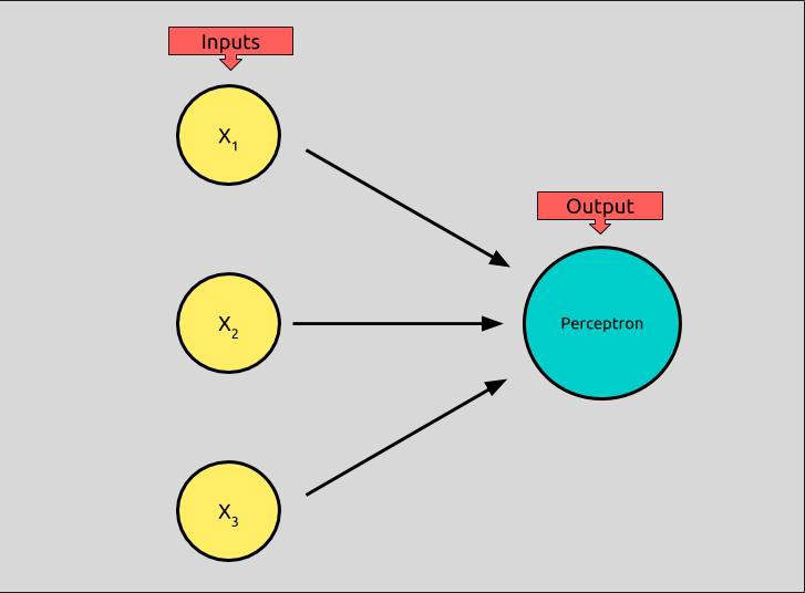
Taken from Michael Nielsen’s Neural Networks and Deep Learning we can model a perceptron that has 3 inputs like this:

A perceptron can have any number of inputs, but this one has three binary inputs x¹, x², and x³, and produces a binary output, which is called its activation.
How can we take three binary inputs and produce one binary output? First, we assign each input a weight, loosely meaning the amount of influence the input has over the output.
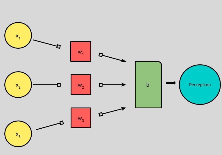
In the picture above, weights are illustrated by black arrows. We’ll call each weight w. Each input, x above has an associated weight: x¹ has a weight w¹, x² a weight of w², and x³, a weight of w³.
To determine the perceptron’s activation, we take the weighted sum of each of the inputs and then determine if it is above or below a certain threshold, or bias, represented by b.
The formula for perceptron neurons can be expressed like this:

Let’s break this down.
-
output is the output of our formula, which is called the activation of our perceptron.
-
Both if branches start with the same ∑ formula which takes each input, x, multiplies it by its weight, w, and then add them all together. This is the weighted sum, in our case, x¹w¹ + x²w² + x³w³, which can also be, (and usually is), represented using dot product notation.
-
If the weighted sum is less than or equal to our threshold, or bias, b, then our output will be 0
-
If the weighted sum is greater than our threshold, or bias, b, then our output will be 1
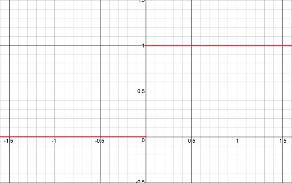
This formula is called a Heaviside Step function, and it can be graphed like this:
f(x) = { x <= b : 0 , x > b : 1 }
Where x is our weighted sum, and b is our bias, 0, in this case.

For any negative x, (input), our y, (output), is 0, and for any positive x, our y is 1.
I want to record this graph, as simple as it is, because it will help demonstrate the differences between perceptrons and sigmoids, later.
(EDIT 25.03.18)
It’s more common to represent the perceptron math like this:

-
The summation is represented using dot product notation.
-
The “threshold” is moved to the other side of the equality and labeled b for “bias.”
-
The summation and bias are added together and compared to 0.
This new way of comparing to 0, offers us a new way of thinking about these artificial neurons. We can think of the bias, now, like a predictor of how easily our neuron will activate, or produce 1 as an output. A neuron with a large bias will indicate that it will “fire” more easily than the same neuron with a smaller bias.
Lastly, pseudocode might look something like this:
def perceptron(inputs, bias)

 weighted_sum = sum {
  for each input in inputs
    input.value * input.weight
  }

  if weighted_sum <= bias
    return 0
  if weighted_sum > bias
    return 1

end
Phew! That was a lot, but now we can add more detail to our perceptron model:

IRL Example
Inspired by the first pages of Michael’s book.
My boyfriend and I want to know whether or not we should make a pizza for dinner. I’m going to rely on our perceptron formula to make a decision. In order to determine if we should make pizza, we’re going to check if we have all of the ingredients, if I’m in the mood for pizza, and if he’s in the mood for pizza.
I really enjoy making pizza, but I hate shopping, so if we don’t have all the ingredients, I’ll only want to make pizza if I’m in the mood for it. If my boyfriend is hungry for pizza, I’ll only want pizza if I don’t have to go to the store, unless I’m also craving pizza.
If, we have all of the ingredients and my boyfriend is in the mood for pizza, but I’m not, we can break down our problem thusly:
Decision:
  Make pizza for dinner?

Inputs:
  x¹ = 1 # We have all of the ingredients.
  x² = 0 # I'm not in the mood for pizza.
  x³ = 1 # My boyfriend is in the mood for pizza.

Weights:
  w¹ = 3 # Having the ingredients makes me willing to have pizza.
  w² = 4 # If I want pizza, I really want pizza!
  w³ = 2 # Him wanting pizza is the least of my concerns.

Bias:
  4
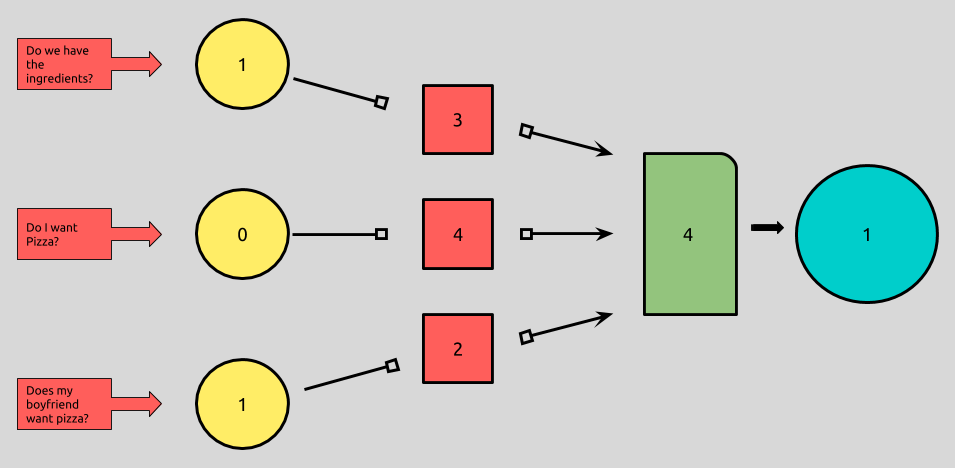
Let’s map it using our illustration!

Each input represents a binary state of each scenario I’m considering, and each weight represents how important each yes-or-no answer is to my final decision. Let’s plug in the numbers.
(1*3) + (0*4) + (1*2) = 5 <= 4 #=> FALSE
(1*3) + (0*4) + (1*2) = 5 <= 4 #=> TRUE = 1
It looks like pizza it is!
Given our perceptron model, there are a few things we could do to affect our output.
If we didn’t have control over out binary inputs, (let’s say they were objective states of being 1 or 0), we could still adjust the weight we give each input, and the bias. For our little pizza question, this is a fun experiment, and could maybe be analogous to how we, as humans, actually solve problems, given objective inputs! We are constantly adjusting the pros-and-cons and priorities we give each input before making a decision.
If I’m not in the mood for pizza, could I still eat it? If yes, then maybe I can decrease the importance of that input. Or maybe, I hate pizza. Then, whether or not I’m in the mood for it should be weighted even higher when it comes to making the decision to have it for dinner or not!
When looking at vanilla neural networks, (multilayer perceptrons), this balancing act is exactly what we’re asking the computer to do. We “train” a network by giving it inputs and expected outputs, and then we ask it to adjust the weights and biases in order to get closer to the expected output, i.e., how can you adjust the weights and biases to get this input, to equal this output?
After we train our network, we then present it inputs it has never seen before. If it’s weights and biases have been calibrated well, it will hopefully begin outputting meaningful “decisions” that has been determined by patterns observed from the many many training examples we’ve presented it.
And this is just the tip of the iceberg.
This is my first journal entry of my dive into machine learning. I’ll list the resources that have gotten me this far, below. Feedback is greatly appreciated, if I’ve gotten something wrong, or taken a misstep, any guidance will be met with open arms!
Thanks for Reading <3