Inspired by biological systems, evolutionary algorithms model the patterns of multi-generational evolution in order to unearth unique ideas. They work by generating a vast number of potential solutions to a particular problem and then pitting them against each other in a process akin natural selection: only the fittest survive. In this way, evolutionary algorithms are able to navigate large ambiguous search spaces in order to find solutions to problems that may be difficult or inefficient to solve using other methods.

These algorithms are used for a wide variety of tasks: from optimizing neural network parameters, evolving mechanical structures, simulating protein folding, and even generating art!

Today, we will use one such algorithm to create a low-poly version of the Ruby logo, using Ruby¹.

Generation: 0000

Max Fitness: 0078.1640

Time (seconds): 0001.03

In this post, we’re going to be using the petri_dish_lab gem for the task of image reconstruction. Image reconstruction is a great example to use because we’ll be able to visualize the evolutionary process working over time.

We’ll begin by going over what an evolutionary algorithm is and how it works. Then, we’ll take a look at the Petri Dish framework and how we can use it to implement an evolutionary algorithm. Next, we’ll define the objective of our image reconstruction problem and how we can represent it in code. Then, we’ll define the genetic operators that we’ll use to evolve the population. Finally, we’ll put it all together and see the results!

🧑‍💻 Code Here
The complete code for this blog post can be found as an example in the examples/low_poly_image_reconstruction directory of the Petri Dish repository.

🔷 What is a Low-Poly Image?
A Low-poly image is a type of 2-D image that’s created by a series of variously sized polygons. Usually, each polygon shares at least one edge with another, and they do not overlap. By using different colors and varying the total polygon count, the result is a low-resolution version of an image.

Table of Contents

• Evolutionary Algorithm Overview
  • The Petri Dish Framework
• Understanding the Objective
• Member Representation
  • Input Target Image
  • Member Genes
  • Reconstructed Output Image
• Population Initialization
• Fitness Function
• Genetic Operators
  • Parent Selection Function
  • Crossover Function
  • Mutation Function
  • Replacement
  • End Condition
• Putting it Together
  • Final Configuration
• Results
  • Subjective Analysis
  • Data Analysis and Interpretation
    • Log Data
    • Image Data
• Conclusion
• Footnotes

Evolutionary Algorithm Overview

Evolutionary algorithms are optimization algorithms that “search” through an expansive space of potential solutions. The goal of a search algorithm is to find a solution that satisfies some criteria, or objective. Evolutionary algorithms are particularly good in cases where we want a solution that is “good enough,” rather than an absolute optimum. In our case, we want to find a set of polygon vertices and grayscale values that, when combined, approximate a given image. For this usecase, there’s no one “best” solution, so evolutionary algorithms are a good fit.

The image reconstruction process begins by creating a bunch of images with random polygons. We’re going to use triangles, but we could technically use any shape, and we’ll stick to grayscale colors in order to make the problem a bit simpler. This collection of images is called the population, and each image is called a member of the population.

Once we have a bunch of random guesses, we compare each member to the target image, pixel-by-pixel, to determine their likeness to the target. This measure of likeness is what we refer to as their fitness, and will be determined by how close each pixel is to the correct grayscale value.

Based on their fitness, parent members are then chosen and combined to create a new child member in a process called crossover. The way we select and crossover parent members is by using selection and crossover functions, and we cover these function (along with mutation functions, which mirror the biological process of genetic mutation by injecting random changes into the child member) later. Together, these functions are called the genetic operators. The exact implementation of these operators is perhaps the most important part of developing an evolutionary algorithm, and we’ll spend a lot of time on them later. If you’re familiar with machine learning, you can think of the genetic operators as hyperparameters.

And, just like in biological systems, the process of parent selection, child creation, and mutation repeats and repeats until we have enough new members to fill a new population. If any of the new members meet our objective, we’re done! Otherwise, we’ll repeat this entire process, known as a generation, until we find a member that meets the objective, or we otherwise get close enough.

An evolutionary algorithm configured in this way is called a genetic algorithm. There are other types of evolutionary algorithms, but they all share a similar recursive structure, shown here in Ruby-esque code:

def run(population = [])
  # If population is empty or not provided, create a new population
  population = Array.new(POPULATION_SIZE) { create_random_member } if population.empty?

  # Try to find a member of the population that meets the objective
  best_member = population.find { |member| objective_met?(member) }

  # If a member meeting the objective is found, return it
  return best_member if best_member

  # Otherwise, create a new generation and recursively search again
  new_population = Array.new(POPULATION_SIZE) do
    parents = select_parents(population)
    child = crossover(parents)
    mutate(child)
  end

  run(new_population)
end

🔄 Tail Call Recursion
Notice that the run method above is recursive. Recursion isn’t always the most efficient way to implement an algorithm because each recursive call in Ruby creates a new stack frame, which is a chunk of memory that stores the state of the method. Depending on how many generations we need our algorithm to run, this could cause an SystemStackError (stack level too deep) error. However, when a recursive call is the last thing that happens in a method (a method returns a call to itself), we can avoid allocating new stack frames by using a technique called tail call optimization. In Ruby, this is not enabled by default, but we can enable it using the following compiler options:

RubyVM::InstructionSequence.compile_option = {
  tailcall_optimization: true,
  trace_instruction: false
}

This prevents the stack from growing indefinitely by reusing the same stack frame for each recursive call, rather than creating a new one.²

The Petri Dish Framework

The Petri Dish framework is a Ruby gem that implements the evolutionary algorithm structure for us in the PetriDish::World.run method. We need to supply the members of the population, how to evaluate their fitness, the genetic operators, and when to stop. These specifics of an evolutionary algorithm are highly dependent on the problem we’re trying to solve, but the underlying structure is always the same.

Here’s what a stripped down version of what the PetriDish::World.run method looks like. See if you can spot the similarities to the pseudocode above:

module PetriDish
  class World
    class << self
      attr_accessor :metadata
      attr_reader :configuration, :end_condition_reached

      def run(
        members:,
        configuration: Configuration.new,
        metadata: Metadata.new
      )
        end_condition_reached = false
        max_generation_reached = false

        max_generation_reached = metadata.generation_count >= configuration.max_generations

        new_members = (configuration.population_size).times.map do
          parents = configuration.parents_selection_function.call(members)
          child_member = configuration.crossover_function.call(parents)
          configuration.mutation_function.call(child_member).tap do |mutated_child|
            end_condition_reached = configuration.end_condition_function.call(mutated_child)
          end
        end

        metadata.increment_generation

        unless end_condition_reached || max_generation_reached
          run(members: new_members, configuration: configuration, metadata: metadata)
        end
      end
    end
  end
end

The PetriDish::World.run method accepts a members Array, which contains the evolving population; a configuration object, which holds the user-defined genetic operators and other configuration options; and an internally used metadata object, which holds information about the current state of the algorithm, like the current generation number.

The Petri Dish framework exposes the PetriDish::Configuration#configure method which takes a block of configuration options.

The core configuration options that we’re interested in for this post are:

We’ll take a look at each of these functions in detail later, but for now, let’s take a step back and define the objective of our problem.

Understanding the Objective

As mentioned earlier, evolutionary algorithms work best when we define a criteria to aim towards, versus a discrete target. In our case, we are trying to replicate a given grayscale image using triangles. If we break this down in terms of drawing polygons, we want to find a set of triangles that, when drawn together, approximate the given image. That is our objective.

We’ll define the triangles by their three vertices. Each vertex can be encoded as an (x,y) coordinate and a grayscale value. These are our decision variables.

A series of these three-vertices-and-a-grayscale-value groupings is all the information we need create a low-poly image. We’ll call these groupings “points” and an Array of them will represent each members’ genes. Each member of the population will have a distinct set of these points and the algorithm will optimize for a member whose points, or genes, are more fit.

☝️ Why Points instead of Triangles?
As we’ll see later, we’ll be using what’s called Delaunay triangulation to create triangles from a member’s points/genes, rather than define triangles directly. Delaunay Triangulation is a technique that takes a set of points and uses them as vertices to creates a set of non-overlapping triangles. This is a creative decision as much as it is a technical one. I began by evolving triangles directly, but found that I didn’t like the results as much as when I evolved points.

Lastly, we need to define our constraints, or the boundaries of the search space. In our case (mostly due to the arbitrary limit of my laptop’s processing power), we will limit the height and width of the image to 100x100 pixels and the color space to 8-bit grayscale. Independently, we will also limit each members’ genes to be 100 points.

🗺️ Quantifying the Search Space
With each point each having an (x,y) coordinate range of (0..100, 0..100) and a grayscale value range of 0..255, each point can be in one of 101 * 101 * 256 = 2,626,816 possible states (roughly speaking). And, since each member has 100 of these as its genes, this leads to a search space of (101 * 101 * 256)**100 dimensions, which is an enormously large, but in practice, quite small for an evolutionary algorithm.

Now that we’ve taken a look at the objective, decision variables, and constraints at a high level, let’s take a look at how we can represent them in code.

To recap:

• Objective: Find a set of non-overlapping triangles that approximate the given image
• Decision Variables: Each vertex can be encoded as an (x,y) coordinate and a grayscale value
• Constraints: 100x100 pixel image, 8-bit grayscale, 100 points

Member Representation

Evolutionary algorithms are generic in the sense that they can be applied to a wide variety of problems. Therefore, just as we would for a neural network, we must engineer, or encode, our problem into a format that can be understood by the algorithm’s architecture.

We need to encode:

1. The input target image,
2. The genes of each member of the population, and
3. The reconstructed output image.

Input Target Image

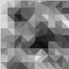
For both the input and output images, we’ll use the Magick gem which provides a Ruby interface to the ImageMagick image processing library.

Starting with an input image path, we can read the image into memory, center crop it to a 100x100 pixel square, and then convert it to grayscale. We’ll save the image to a file for later comparison.

require 'rmagick'

def import_target_image(input_path, output_path)
  image = Magick::Image.read(input_path).first

  # Calculate crop size and coordinates for center crop
  crop_size = [image.columns, image.rows].min
  crop_x = (image.columns - crop_size) / 2
  crop_y = (image.rows - crop_size) / 2

  image
    .crop(crop_x, crop_y, crop_size, crop_size)
    .resize(IMAGE_HEIGHT_PX, IMAGE_WIDTH_PX)
    .quantize(256, Magick::GRAYColorspace)
    .write(output_path)

  image
end

Let’s import the Ruby logo and see what it looks like:

IMAGE_WIDTH_PX = 100
IMAGE_HEIGHT_PX = 100

target_image = import_target_image("ruby_logo.png", "ruby_logo_grayscale.png")

Using the Magick::Image class to represent our target image is arbitrary, but the rmagick library provides a convenient interface for reading, writing, and importantly, comparing images pixel-by-pixel. (We’ll use this later to calculate the fitness of each member).

Member Genes

When defining of our objective, we identified that the genes of each member can be represented as an Array of 100 points, each with an (x,y) coordinate and a grayscale value that defines the vertices of triangles. We can encode this using a Point Struct with x, y, and grayscale attributes.

Point = Struct.new(:x, :y, :grayscale)

📐 Why a Struct?
A Struct is a simple way to define a class with attributes. It’s a good choice here because we do not need to define any behavior on Point-s; it is a data-only object. Based on my benchmarks³, a hash would be more performant, through it’s less flexible and less explicit. A class or Ruby 3.2 Data object offer no additional benefits.

🌈 Why does a Point have color?
Notice here that a the grayscale attribute is defined on the Point Struct and not on some representation of a triangle. We’ll need a grayscale value to fill each triangle, but a triangle will be made up of three Point-s. So, which of the three Point-s’ grayscale attribute do we use? We will average them. This is because, as we will see, we aren’t sure which three Point-s will be used together as the vertices of any particular triangle. Therefore, for any given triangle, we’ll average the grayscale values of its three Point-s together to determine the fill color. This is only one approach to this problem.

Now that we have a Point, we can create an Array of them to form a member’s genes.

The Petri Dish framework provides a PetriDish::Member class, which acts as an interface to the library. The PetriDish::Member class holds onto the genes Array, which is then directly exposed via the PetriDish::Member#genes method.

Here is the entire definition of the PetriDish::Member class:

module PetriDish
  class Member
    attr_reader :genes

    def initialize(genes:, fitness_function:)
      @fitness_function = fitness_function
      @genes = genes
    end

    def fitness
      @fitness ||= @fitness_function.call(self)
    end
  end
end

The initializer also accepts a fitness_function which is used to evaluate the fitness of a member. (We’ll define the fitness function later, but for now, it only needs to respond to #call and take a PetriDish::Member as its only argument).

To create a PetriDish::Member with an Array of 100 random Point-s as its genes, we do the following:

GRAYSCALE_RANGE = 0..255

def random_member
  genes = Array.new(100) do
    Point.new(rand(0..IMAGE_WIDTH_PX), rand(0..IMAGE_HEIGHT_PX), rand(GRAYSCALE_RANGE))
  end

  PetriDish::Member.new(genes: genes, fitness_function: ->(_member) { })
end

puts random_member.genes.sample(3)
#<struct Point x=57, y=21, grayscale=235>
#<struct Point x=16, y=49, grayscale=64>
#<struct Point x=68, y=6, grayscale=210>

Reconstructed Output Image

To turn a PetriDish::Member into a low-poly image, we’ll create triangles using its #genes in a process called Delaunay triangulation. This technique takes a set of points and creates a set of triangles such that no point is inside the circumcircle of any triangle, i.e. no triangle overlaps another. The delaunator gem is a Ruby library that performs Delaunay triangulation, and we’ll use it here instead of implementing it ourselves.

Let’s define a function called member_to_image that takes a PetriDish::Member and returns an Magick::Image object based on the member’s genes (while also grossly violating the single-responsibility principle).

1. We begin by initializing a new Magick::Image object, which is the same object type as our input image.
2. We then perform the Delaunay triangulation using the Delaunator.triangulate method and passing in the x and y values from the Point-s returned from the PetriDish::Member#genes method.
3. To determine the grayscale fill value, we use the grayscale value from PetriDish::Member#genes, and average them, as we discussed earlier.
4. Finally, we draw each triangle onto the image using the Magick::Draw#polygon method.

require 'petri_dish'
require 'delaunator'

def member_to_image(member)
  # Create a new image with a white background
  image = Magick::Image.new(IMAGE_WIDTH_PX, IMAGE_HEIGHT_PX) { |options| options.background_color = "white" }

  # Create a new draw object to draw onto the image
  draw = Magick::Draw.new

  # Perform Delaunay triangulation on the points
  #
  # Delaunator.triangulate accepts a nested array of [[x1, y1], [xN, yN]]
  # coordinates and returns an array of triangle vertex indices where each
  # group of three numbers forms a triangle
  triangles = Delaunator.triangulate(member.genes.map { |point| [point.x, point.y] })

  triangles.each_slice(3) do |i, j, k|
    # Get the vertices of the triangle
    triangle_points = member.genes.values_at(i, j, k)

    # Use the average color from all three points as the fill color
    color = triangle_points.map(&:grayscale).sum / 3

    # The `Magick::Draw#fill` method accepts a string representing a color in the form "rgb(r, g, b)"
    draw.fill("rgb(#{color}, #{color}, #{color})")

    # Magick::Image#draw takes an array of vertices in the form [x1, y1,..., xN, yN]
    vertices = triangle_points.map { |point| [point.x, point.y] }
    draw.polygon(*vertices.flatten)
  end

  draw.draw(image)
  image
end

Let’s see what the result looks like if we run it a few times:

5.times do |i|
  member_to_image(random_member).write("member#{i}.png")
end

Here, we can see the Delaunay triangulation in action. Each member has a different set of points, and therefore a different set of triangles. We can also see that the grayscale values are being averaged together to determine the fill color of each triangle.

When we use an Magick::Image object to represent a member of the population, we do so to easily compare it to the Magick::Image target object and visualize the results from the algorithm.

When we use the Petridish::Member object to represent the same member, we do so to enable the algorithm to easily calculate and evolve new members.

This type of data engineering, akin to feature engineering in machine learning, is a critical step in the process of developing an evolutionary algorithm. The way we encode the problem and represent potential solutions has a large impact on the performance of the algorithm and our ability to interpret its output.

⬜️ Why the White Background?
When we create a new Magick::Image object to represent a member in the member_to_image method, we opt for white as the background color. This choice, although arbitrary, influences the performance of the algorithm. For instance, with the grayscale Ruby logo, whose background is largely white, starting with a white background might expedite the convergence on a solution. However, hardcoding this value may bias the algorithm towards reconstructing targets with white backgrounds. The best solution would be to make this choice configurable in order to make this parameter tunable. This is a good example of how the smallest details in the way we model a problem can impact the performance of the algorithm.

Population Initialization

Often it is the case that completely random population initialization is a good place to start, but we can sometimes quickly see faster results if seed the population with some prior knowledge; similar to choosing a good initial set of weights for a neural network.

In the case of image reconstruction, I found that random initialization lead to a lot of waste in the early generations on distributing the points across the image dimensions. To avoid this, we can instead evenly distribute the points across the x and y dimensions of the image and then randomly assign a grayscale value to each point.

def init_member
  PetriDish::Member.new(
    genes: (0..IMAGE_WIDTH_PX).step(10).map do |x|
              (0..IMAGE_HEIGHT_PX).step(10).map do |y|
                Point.new(x, y, GRAYSCALE_VALUES.sample)
              end
            end.flatten,
    fitness_function: ->(_member) { }
  )
end

Let’s see what the result looks like if we run this method a few times:

5.times do |i|
  member_to_image(init_member).write("member#{i}.png")
end

We can see that the points are evenly distributed across the image dimensions, and that the grayscale values are randomly assigned. Whether or not this is a better starting point than a completely random initialization is a question of experimentation. In the case of image reconstruction and other generative tasks, a random initialization may be better because it allows the algorithm to explore the search space more creatively, though it may take longer to converge on a solution.

Fitness Function

The fitness function is a function that takes a Member and returns a number that represents how well that member solves the problem. In our case, we want to know how well a member approximates the target image.

Modeling a fitness function to map to the search space is often the most difficult part of developing an evolutionary algorithm. It’s also the most important part because it’s what the algorithm uses to determine which members are better than others. Two key qualities of a fitness function are determinism and discrimination.

Deterministic means that given the same Member, the fitness function should always return the same fitness score. This is because the fitness of a member may be evaluated multiple times during the evolutionary process, and inconsistent results could lead to unpredictable behavior.

Discriminative means that the fitness function should be able to discriminate between different members of the population. That is, members with different genes should have different fitness scores. Although fitness function do not have to be strictly discriminative, if many members have the same fitness score, the evolutionary algorithm may have a harder time deciding which members are better.

Lucky for us, the rmagick library provides an Image#difference method that fits the bill. Image#difference compares two images and returns three numbers that represent how different they are: mean_erorr_per_pixel, normalized_mean_error, and normalized_maximum_error. We’ll use the normalized_mean_error to calculate our fitness score.⁴

require 'petri_dish'
require 'rmagick'

  def calculate_fitness(target_image)
    ->(member) do
      member_image = member_to_image(member, IMAGE_WIDTH_PX, IMAGE_HEIGHT_PX)
      # Magick::Image#difference returns a tuple of:
      # [mean error per pixel, normalized mean error, normalized maximum error]
      (1.0 / target_image.difference(member_image)[1])**2 # Use normalized mean error
    end
  end

The fitness function is a lambda that takes a Member and returns a fitness score. The number is the inverse of the normalized mean error between the target image and the image generated from the member, squared. This means that the higher the fitness score, the better the member approximates the target image.

🎛️ Why normalized?
The normalized mean error is a number between 0 and 1 that represents the average difference between the grayscale values of each pixel in the target image and the member image. This puts the error of every member on the same scale. When comparing members that all have the same dimension and color scale, normalization may be moot, but sneakily, we can reuse this fitness function for other images that may have different dimensions and color scales and generally compare the performance of the algorithm across those different target images.

🙃 Why the inverse?
When the normalized mean error is inverted (i.e., 1 divided by the normalized mean error), we get a fitness score such that smaller errors (which are closer to 0 after normalization) yield larger fitness values, and larger errors yield smaller fitness values. This means the less “wrong” a member is, the higher its fitness will be.⁵

2️⃣ Why squared?
In effect, this transformation makes our algorithm very sensitive to the quality of the solutions. Solutions that are closer to the target (i.e., have a larger inverted normalized mean error) are assigned significantly higher fitness scores, and are therefore more likely to be selected for reproduction in the next generation (generally true, but depending on the selection function we define later). This can potentially speed up convergence, but as always, we should be cautious of premature convergence on sub-optimal solutions if there is not enough diversity in the population.

Lastly, we define #calculate_fitness as a lambda because the Petri Dish framework requires the fitness_function to respond to #call. The framework will call this lambda via the #fitness method on Member in order to memoize and return the fitness score. We use a closure here so that the target_image is available to the lambda when it’s called.

📫 Closures
Closures are a powerful feature of Ruby and other languages. They allow us to define a function that can be called later, but that also has access to the variables that were in scope when the function was defined. It’s like putting a note inside an envelope for the function to open later. In our case, we want to define a function that can be called later by the Petri Dish framework, but that also has access to the target_image that we defined earlier.

Now that we have a way to represent a member of the population and a way to evaluate the fitness of a member, we can start to evolve the population by defining the evolutionary operators.

Genetic Operators

The genetic operators are the functions that we use to evolve the population generation after generation—they are what allow the algorithm to navigate the vast search space of potential solutions.

The operators we’ll take a look at are grouped by selection, crossover, mutation, and replacement.

Parent Selection Function

Selection is the process of choosing which members of the population are the most fit and therefore should be used as parents to create the next generation of children. There are many different selection strategies, but for our task, we’ll use one called fitness proportionate selection.

Also called roulette wheel selection or stochastic acceptance, fitness proportionate selection works by assigning each member a weighted probability of being selected as a parent, and then randomly selects parents based on those probabilities.

The weighted probability assigned to each member is proportional to that member’s fitness score, which means that members with higher fitness scores are more likely to be selected.

For example, let’s say we have the following Member-s with the following fitness scores:

population = [
  Member.new(genes: [1, 2, 3], fitness_function: ->(_member) { 2 }),
  Member.new(genes: [4, 5, 6], fitness_function: ->(_member) { 3 }),
  Member.new(genes: [7, 8, 9], fitness_function: ->(_member) { 5 }),
]

To calculate the proportional fitness for each member, we divide the member’s fitness by the total fitness of the population. In our case, the total fitness is 2 + 3 + 5 = 10. Dividing each members’ fitness by this number gives us the proportion of the total fitness that that member contributes.

If we calculate a proportional fitness for each member from our example, we get the following results:

weights = population.map { |member| member.fitness / population.sum(&:fitness).to_f }
# => [0.2, 0.3, 0.5]

In our example, if we were to select multiple members using these weighted probabilities, we would expect to get the first member (population[0]) 20% of the time, the second member (population[1]) 30% of the time, and the third member (population[2]) 50% of the time.

We can then use these proportional fitnesses, to weigh, or bias the otherwise equally random probability of each member being selected.

Here’s what that looks like:

  def roulette_wheel_parent_selection_function
    ->(members) do
      population_fitness = members.sum(&:fitness)
      members.max_by(2) do |member|
        weighted_fitness = member.fitness / population_fitness.to_f
        rand**(1.0 / weighted_fitness)
      end
    end
  end

The proportional fitness is calculated by dividing the member’s fitness by the total population fitness, like before. Then, we raise a random number between 0 and 1 to the inverse of the proportional fitness in order to bias the selection towards members with higher fitness scores. The Enumberable#max_by method is used to select two members with the highest result from the block.

The maths are a bit annoying to me personally, but nevertheless, the result of all of this is like spinning a roulette wheel where the size of each slice is proportional to the member’s fitness. The higher the fitness, the larger the slice, and the more likely the member is to be selected.

Notice how the parent selection function makes no mention of Point-s or Magick::Image-s. This is because the selection function is generic and can be used for any problem. It only needs to know how to select members based on their fitness scores.

There are many other selection methods, like simply selecting the fittest members (elite selection) or by first choosing a random subset of the population and then choosing the fittest amongst those (tournament selection).

The benefit of fitness proportional selection is that it allows for a balance between exploration (trying new things) and exploitation (using what we know works). This is because members with lower fitness scores still have a chance of being selected, but members with higher fitness scores are more likely to be selected.

This is the selection method we’ll use for our task, but it may be worth experimenting with other selection methods to see if they work better for our problem.

👨‍👨‍👦 Multiple Parents
Although most implementations of evolutionary algorithms that I’ve seen select two parents, it is possible to select more than two. In fact, the Petri Dish framework allows for any number of parents to be inside the Array returned by the selection function lambda.

Crossover Function

In biology, crossover is when paired chromosomes from each parent swap segments of their DNA. This creates new combinations of genes, leading to genetic diversity in offspring. In evolutionary algorithms, crossover is the process of combining the genes of parents members to create a new child member.

After selecting parents, their genes, an Array of Point-s in our case, are combined to create a new Petridish::Member. There are many different ways to combine the genes of parents, but for our task, we’ll use a method called random midpoint crossover to crossover two parents.

Random midpoint crossover works by randomly selecting a midpoint in the genes of each parent and then combining the genes before and after that midpoint to create a new child. Specifically, we’ll randomly select a midpoint between 0 and the length of the genes Array, and then take the genes before that midpoint from the first parent and the genes after that midpoint from the second parent.

For example, say we have two parents with the following genes:

parent_1 = PetriDish::Member.new(
  genes: [
    Point.new(1, 2, 25),
    Point.new(3, 4, 50),
    Point.new(5, 6, 100),
  ],
  # fitness_function: ...
)
parent_2 = PetriDish::Member.new(
  genes: [
    Point.new(7, 9, 125),
    Point.new(9, 10, 150),
    Point.new(11, 12, 200),
  ],
  # fitness_function: ...
)

If we were to perform random midpoint crossover on these parents, and the midpoint = 1, we would get the following child:

child = PetriDish::Member.new(
  genes: [
    Point.new(1, 2, 25),
    Point.new(9, 10, 50),
    Point.new(11, 12, 200),
  ],
  # fitness_function: ...
)

Here’s our random_midpoint_crossover_function implementation for combining two parents:

  def random_midpoint_crossover_function(configuration)
    ->(parents) do
      midpoint = rand(parents[0].genes.length)
      PetriDish::Member.new(genes: parents[0].genes[0...midpoint] + parents[1].genes[midpoint..], fitness_function: configuration.fitness_function)
    end
  end

Note again, our function returns a lambda, as required by the Petri Dish framework. The lambda takes an Array of parents and returns a new PetriDish::Member with the combined genes of the parents, while also passing along the fitness_function from the configuration object captured by the closure. As before, the fitness function works generically and does not need to know about Point-s or Magick::Image-s.

Other crossover methods include uniform crossover, where each gene is randomly selected from either parent, and majority rule crossover, which works well for instances of selecting more than two parents. It works by having each gene of the offspring determined by a majority vote among the parents. If the parents have equal votes, one parent is chosen randomly to determine the gene.

Random midpoint crossover is a good choice for starting out for its simplicity, but again, it’s worth experimenting with other crossover methods to see if they work better for a particular problem. (In fact, its possible to use one genetic algorithm to optimize the genetic operators of another genetic algorithm, but that’s a topic for another day…).

👩‍🔬 Meta Experimentation
This type of meta experimentation is akin to hyperparameter tuning in machine learning. A core design philosophy of the Petri Dish framework is to make it easy to experiment with different configurations in this way. By passing in different functions for the genetic operators, we can easily experiment with different configurations and observe which ones work best.

That said, for our task, random midpoint crossover works well enough, so we’ll stick with it for now.

Mutation Function

Mutation is the process of randomly changing the genes of a child member after crossover. Combining well-fit parents can get us a long way towards a great solution, but mutation is done to introduce new genetic material into the population.

There are many different ways to mutate a member, but for our task, we’ll use a domain-specific implementation that I call nudge mutation.

🧬 Why mutate at all?
Mutation is not strictly necessary for an evolutionary algorithm to work. However, mutation increases diversity and diversity is what allows the algorithm to explore the search space more thoroughly. Without mutation, the algorithm may get stuck in a local maximum, i.e. be unable to find a better solution, though one may exist. Mutation allows the algorithm to escape this local maximum and continue searching for a better solution.

If we think back to our genes as an Array of Point-s, then nudge mutation is the process of randomly moving each point’s position and grayscale value by a small amount.

This is done by adding a random number between -10 and 10 to the x and y coordinates of each point clamp-ed between the image dimensions. And, adding a random number between -25 and +25 to the grayscale value clamp-ed between 0..255 (i.e. valid grayscale values).

If we implemented this as a lambda for the Petri Dish mutation_function configuration (RBS type Proc[Member, Member]), it might look something like this:

  def nudge_mutation_function(configuration)
    ->(member) do
      mutated_genes = member.genes.dup.map do |gene|
        Point.new(
          (gene.x + rand(-10..10)).clamp(0, IMAGE_WIDTH_PX),
          (gene.y + rand(-10..10)).clamp(0, IMAGE_HEIGHT_PX),
          (gene.grayscale + rand(-25..25)).clamp(GRAYSCALE.min, GRAYSCALE_RANGE.max)
        )
        end
      PetriDish::Member.new(genes: mutated_genes, fitness_function: configuration.fitness_function)
    end
  end

However, we don’t want to mutate every gene of a child; we want to preserve qualities from the parents and strike a balance between exploration and exploitation. Therefore, we use a mutation rate to determine the probability that any particular gene will be mutated.

For example, if the mutation rate is 0.1, then there is a 10% chance that a gene will be mutated.

If we add the concept of a mutation rate to our mutation function, we get this:

def nudge_mutation_function(configuration)
  ->(member) do
    mutated_genes = member.genes.dup.map do |gene|
+      if rand < configuration.mutation_rate
        Point.new(
          (gene.x + rand(-10..10)).clamp(0, IMAGE_WIDTH_PX),
          (gene.y + rand(-10..10)).clamp(0, IMAGE_HEIGHT_PX),
          (gene.grayscale + rand(-25..25)).clamp(GRAYSCALE.min, GRAYSCALE_RANGE.max)
        )
+      else
+        gene
+      end
    end
    PetriDish::Member.new(genes: mutated_genes, fitness_function: configuration.fitness_function)
  end
end

Here, we use the configuration.mutation_rate to determine whether or not to mutate each gene. If the random number is less than the mutation rate, we mutate the gene, otherwise, copy it over to the new PetriDish::Member as-is.

📈 Determining the mutation rate
The mutation rate is a hyperparameter that can be tuned to improve the performance of the algorithm. A higher mutation rate will increase diversity, but it may also cause the algorithm to take longer to converge. A lower mutation rate will decrease diversity, but it may also cause the algorithm to get stuck in a local maximum. The mutation rate is often a good hyperparameter to tune when trying to improve the performance of an evolutionary algorithm.⁶

Other common types of mutation strategies include swap mutation, where two genes’ positions are randomly swapped, and scramble mutation, where a random subset of genes are randomly shuffled. Like all other genetic operators, the best strategy for the problem at hand is highly dependent on the problem itself and is often worth experimenting with.

In our case, the mutation function implementation was developed to represent the idea of nudging around the points of a polygon until the resulting image looks like the target image.

🪲 Point jitter??
You may see that in the actual implementation of this method, I’ve added a point_jitter of rand(-0.0001..0.0001) to each x and y of Point. This is because the particular implementation of the Delaunay algorithm would fall into a divide-by-zero error if all of the points were collinear (on exactly on the same line). This is a good example of how reality is often messier than theory, and how we must adapt our models and implementation to the problem at hand.

Now that we have a way to select parents, combine their genes, and mutate the resulting child, we can start to evolve the population. The last step is to define how we’ll replace the old population with the new population.

Replacement

In the most simple case, we can replace the entire population with the new population, sometimes called generational replacement. This often works well, but it can sometimes cause too much diversity, which can cause the algorithm to take longer to converge as some of the most-fit members are lost. To prevent this, we can use a technique called elitism.

Elitism, which I personally like to call grandparenting, is the process of preserving the fittest members of the population from one generation to the next. This is done by taking the top n members of the population and adding them to the new population. The rest of the new population is filled with the children of the parents.

In the Petri Dish framework, we tune this parameter using the elitism_rate configuration value. This is the proportion of the population that is preserved through elitism. For example, if the elitism rate is 0.1, then the top 10% of the population will be preserved through to the next generation.

Other replacement strategies include steady-state replacement, where only a single member of the population is replaced with a child, and age-based replacement, where the oldest members of the population are replaced with children.

For our image reconstruction task, we’ll use generational replacement with grandparenting set to 0.05, or 5%.

End Condition

Lastly, we need to define when the algorithm should stop. The two most common end conditions are 1) when a member of the population meets the criteria, or 2) when a certain number of generations have passed. We’ll use the latter.

An end_condition_function can otherwise be used to determine if any of the members of the population meets a particular criteria. For example, if we were trying to find a member of the population that had a fitness score of 1.0, we could use an end_condition_function. Alternatively, we could run the algorithm for a given amount of wall time, or until the rate of improvement drops below a certain threshold.

In our case, we’ll use the max_generations configuration value to determine when the algorithm should stop. This is the maximum number of generations that the algorithm will run for, regardless of the fitness of the members of the population. I have found that 5000 generations is enough to get a good approximation of the target image, but not so many that it takes too long to run.

We now have all of the pieces we need to put together our evolutionary algorithm. Let’s see how it all works!

Putting it Together

Before we look at the results, let’s recap everything we’ve gone over.

1. A genetic algorithm is a type of evolutionary algorithm that uses genetic operators to evolve a population of members towards a solution to a problem.
2. We start the algorithm design by identifying our objective, defining our decision variables and search space, and defining our constraints.
3. We then define a way to represent a member of the population and a way to evaluate the fitness of a member.
   1. In our case, we represent a member of the population as an Magick::Image object, and we evaluate the fitness of a member by comparing it to the target image using the Magick::Image#difference method.
   2. We also represent a member of the population as a PetriDish::Member object with an Array of Point-s as genes, which is used by the Petri Dish framework to evolve the population.
4. The genetic operators are selection, crossover, mutation, and replacement.
   1. Selection is the process of choosing which members of the population are the most fit and therefore should be used as parents to create the next generation of children.
   2. Crossover is the process of combining the genes of parents members to create a new child member.
   3. Mutation is the process of randomly changing the genes of a child member after crossover.
   4. Replacement is the process of replacing the old population with the new population.
5. The end condition is the criteria that determines when the algorithm should stop.
   1. In our case, we’ll use the max_generations configuration value to determine when the algorithm should stop. This is the maximum number of generations that the algorithm will run for, regardless of the fitness of the members of the population.

Final Configuration

The following is the configuration from the actual implementation and contains all of the pieces we’ve discussed so far, with the addition of a few callbacks that the framework provides.

def configuration
  PetriDish::Configuration.configure do |config|
    config.population_size = 50
    config.mutation_rate = 0.05
    config.elitism_rate = 0.05
    config.max_generations = 10_000
    config.fitness_function = calculate_fitness(target_image)
    config.parents_selection_function = roulette_wheel_parent_selection_function
    config.crossover_function = random_midpoint_crossover_function(config)
    config.mutation_function = nudge_mutation_function(config)
    # TODO: Don't pass in image dimensions, use constants instead
    config.highest_fitness_callback = ->(member) { save_image(member_to_image(member, IMAGE_WIDTH_PX, IMAGE_HEIGHT_PX)) }
    config.generation_start_callback = ->(current_generation) { generation_start_callback(current_generation) }
    config.end_condition_function = nil
  end
end

The highest_fitness_callback is invoked when a member with the highest fitness seen so far is found. When that happens, we save the image to a file so that we can see the progress of the algorithm.

The generation_start_callback is invoked at the start of each generation. We use this to keep track of the progress of the algorithm to do things like name the output images.

The last piece of the configuration we haven’t discussed yet is the population_size. This is the number of members in the population per generation, and like all other pieces of configuration, is a hyperparameter that should be tuned to improve the performance of the algorithm. A larger population size can increase diversity, but it may also cause the algorithm to take longer to converge. A smaller population size can decrease diversity, but can be aided with a higher mutation rate and maximum number of generations, as we’ve done here.

Results

Finally, it’s time to run the algorithm and see what happens! Let’s take a subjective look at the results before we get into the numbers.

Generation: 0000

Max Fitness: 0078.1640

Time (seconds): 0001.03

Subjective Analysis

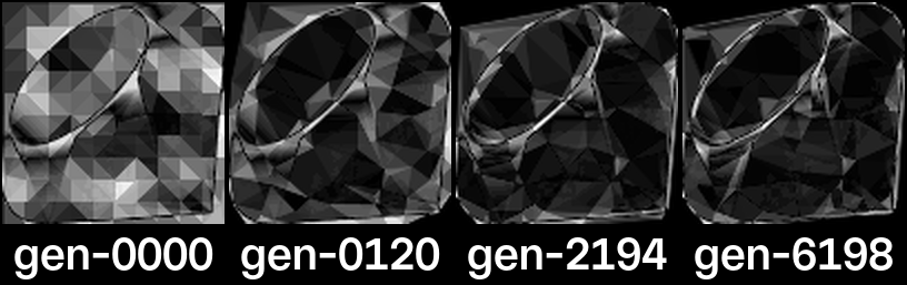
After running the algorithm for over 6000 generations over the course of an hour, I’m really please with the results!

I’m surprised by the details the algorithm was able to replicate. For example, the curvature of the top of the ruby is really well defined, given that we’re working with only straight lines. Also, the highlights along the gem’s facets were captured well. If I squint hard enough, I have a hard time distinguishing the target image from the result!

With that said, there are some points stuck in the upper left corner that are shading part of the background the wrong color, but I think it’s those points are actually contributing to the gem’s curvature that I mentioned earlier.

It looks like algorithm had a lot of early success: by generation 120, we can already begin to see vast improvements! However, as the algorithm continued to run, the gains each generation appeared to diminish, which is to be expected from an evolutionary algorithm and an exponential fitness function. After about generation 2000, the algorithm was making smaller and smaller tweaks to the image.

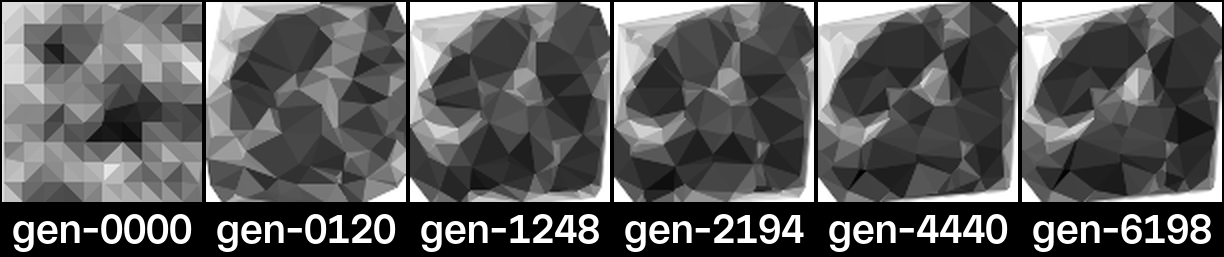
The biggest improvements to the image after the early generations appear to be in the grayscale values, rather than the positions of the points. This makes sense because the position of the points only really matter in that the resulting triangle contributes to the grayscale value of the pixels it covers.

By looking only at the images, it’s hard for me to tell how much the algorithm improved after generation 2000 and wether or not we could have stopped it there.

I’m curious to see if the numbers tell a different story.⁷

Data Analysis and Interpretation

Now that we’ve taken a subjective look at the results, let’s take an objective look at the algorithm’s performance. We’re going to take these numbers with a grain of salt: since we’ve only ran the algorithm once and with one set of configurations, there is nothing to characterize the performance against.⁸ Additionally, we’re going to look at the numbers from the perspective of the algorithm’s performance only, rather than the performance of the Ruby code itself^{9 10}

Log Data

I, [2023-08-04T19:48:28.744335 #83090]  INFO -- : {"id":"869b3cc4-b37b-47ff-8beb-602aaa52c48f","generation_count":0,"highest_fitness":0,"elapsed_time":0.0,"last_fitness_increase":0}
I, [2023-08-04T19:48:29.393945 #83090]  INFO -- : {"id":"869b3cc4-b37b-47ff-8beb-602aaa52c48f","generation_count":0,"highest_fitness":45.43454105775939,"elapsed_time":0.65,"last_fitness_increase":0}
I, [2023-08-04T19:48:29.422413 #83090]  INFO -- : {"id":"869b3cc4-b37b-47ff-8beb-602aaa52c48f","generation_count":0,"highest_fitness":73.14234456163621,"elapsed_time":0.68,"last_fitness_increase":0}
I, [2023-08-04T19:48:29.702998 #83090]  INFO -- : {"id":"869b3cc4-b37b-47ff-8beb-602aaa52c48f","generation_count":0,"highest_fitness":75.73263190998411,"elapsed_time":0.96,"last_fitness_increase":0}
I, [2023-08-04T19:48:29.775709 #83090]  INFO -- : {"id":"869b3cc4-b37b-47ff-8beb-602aaa52c48f","generation_count":0,"highest_fitness":78.16397715764293,"elapsed_time":1.03,"last_fitness_increase":0}
I, [2023-08-04T19:48:29.990462 #83090]  INFO -- : {"id":"869b3cc4-b37b-47ff-8beb-602aaa52c48f","generation_count":1,"highest_fitness":78.16397715764293,"elapsed_time":1.25,"last_fitness_increase":0}
I, [2023-08-04T19:48:30.146199 #83090]  INFO -- : {"id":"869b3cc4-b37b-47ff-8beb-602aaa52c48f","generation_count":1,"highest_fitness":85.22354925417734,"elapsed_time":1.4,"last_fitness_increase":1}
I, [2023-08-04T19:48:30.543062 #83090]  INFO -- : {"id":"869b3cc4-b37b-47ff-8beb-602aaa52c48f","generation_count":2,"highest_fitness":85.22354925417734,"elapsed_time":1.8,"last_fitness_increase":1}
I, [2023-08-04T19:48:30.711047 #83090]  INFO -- : {"id":"869b3cc4-b37b-47ff-8beb-602aaa52c48f","generation_count":2,"highest_fitness":95.88177285281498,"elapsed_time":1.97,"last_fitness_increase":2}
I, [2023-08-04T19:48:31.090201 #83090]  INFO -- : {"id":"869b3cc4-b37b-47ff-8beb-602aaa52c48f","generation_count":3,"highest_fitness":95.88177285281498,"elapsed_time":2.35,"last_fitness_increase":2}
I, [2023-08-04T19:48:31.405858 #83090]  INFO -- : {"id":"869b3cc4-b37b-47ff-8beb-602aaa52c48f","generation_count":3,"highest_fitness":100.92915163430119,"elapsed_time":2.66,"last_fitness_increase":3}

Using the logs as a data source, let’s start by looking at a plot of the highest fitness score of any population over time. The fitness was determined by the inverse of the normalized mean error between the target image and the image generated from the member, squared. The higher the fitness, the better the member approximates the target image.

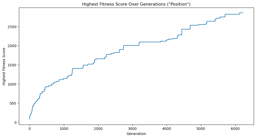
We can see that the fitness of the fittest member of each population trends heavily positive over time; somewhat linearly but with a steeper slope at the beginning. This is to be expected because the algorithm starts with a lot to gain from its initial, somewhat random, initial state, and then spends time improving on better and better results.

We can also see that the the trend is not monotonically increasing, i.e. it does not always increase from one time step (generation) to the next. This is because the algorithm is not guaranteed to find a better solution in each generation.

We can visualize this by plotting the change in highest fitness over time, which I called velocity, but can also be considered efficiency.

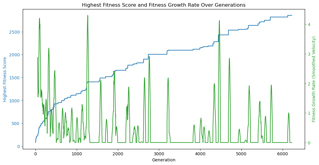
Here, we can see a lot of zero-efficiency/zero-velocity generations, where the fitness of the fittest member of the population did not change from the previous generation, specifically after about the 1000th generation. This shows us in another way that the algorithm is converging on a solution.

In fact, we could this metric to improve our end condition function, i.e. stop the algorithm when the efficiency drops below a certain threshold, rather than blindly after a certain number generations or a particular fitness score. We can also use efficiency to compare the performance of different configurations.

That said, convergence on a solution doesn’t always mean that the solution is the best solution to be found, just that it’s the best so far. We should be careful not to prematurely stop the algorithm. For example, at around generation 4500, we see another significant spike in efficiency even after many hundreds of generations with little-or-no improvement.

Image Data

Subjectively, I thought that there was little to be gained after generation 2000, but based on the data from the logs, we know that the algorithm continued to find fitter members, almost linearly! Is generation 6198, with a fitness score of 2857.08, really 68% better than generation 2194 with a fitness score of 1700.74?

What does “68% better” look like?

Let’s start by taking a look at the error across individual pixels. If we remember back to our fitness function, we know that the fitness score was determined by the mean error of each pixel, i.e. how far off the grayscale value of each pixel was from the target image. We can visualize this by plotting the grayscale value of a few random pixel over time.

Here, we’re plotting the same five pixels from each member as they journey towards their target (indicated by the dashed lines) over each generation. We can observe that these pixels remain relatively stable after just a few hundred generations, and even more so after about 2500 generations. We can also notice that while some pixels hit their target dead on, others get farther away over time.

Interestingly, we can see some pixels correlate to the global trends we saw in the log data earlier: pixel 4 makes a significant improvement around generation 2500, and pixel 1 makes a significant improvement around generation 4500.

We see a similar story when we look at 10 pixels near the center of the image that are all moving towards the same grayscale value. Looking at neighboring pixels is interesting because the algorithm is evolving the population by moving the vertices of triangles around, and therefore, the grayscale values of neighboring pixels are likely to be correlated.

Again, we can see that the pixels stabilize after about 250 generations, even more so after around after 2500. And, we also clearly see the correlation to the large spike around generation 4500 that we saw in the log data. It appears that these pixels were somewhat stuck for over 1000 generations, and then suddenly jumped to their target grayscale value. Curiously, we can also see a divergence after 5500 generations, even though the overall fitness score continued to increase…

If we render the differences between the target image and a sample of generations, we get the images above. In these images, the darker the pixel, the closer the grayscale value of the pixel is to the target image.

This is a good way to visualize our fitness function as the algorithm is essentially trying to increase the number of black pixels and decrease the number of white pixels. We can see that the differences are, in fact, decreasing over time, but it’s still hard to see the 68% difference between generations 2194 and 6198.

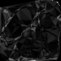
If we look at the difference of the differences between generations 2194 and 6198, we see mostly dark colored pixels, indicating that the differences are small, and perhaps nearly imperceptible.

This is what “68% better” looks like!

Despite all the math and theory, throughout this exploration, we have aimed the power of evolutionary algorithms towards scratching the subjective search space surface of creativity and art. Algorithmic processes can produce results that are not only fascinating from a technical standpoint but also visually (and philosophically) compelling. At the end of analyzing our algorithm’s ability to near its target, we are left to contemplate how well the resulting image captures our aesthics and creative vision.

Conclusion

Crafting a low-poly image representation is but one example of the myriad applications of evolutionary algorithms. The /examples directory within the Petri Dish repository showcases additional uses, including tackling the Travelling Salesperson Problem and a more straightforward task of text generation.

Despite the diverse applications, evolutionary algorithms generally follow a uniform framework, as discussed in Putting it Together. Interestingly, many of the design considerations we covered in this blog post are even more broadly applicable to the field of data engineering.

If you’re intersted in exploring the use of genetic algorithms for creative purposes, I can recommend:

• “The Nature of Code” by Daniel Shiffman, particularly the chapters on evolutionary algorithms.
• “Generative Art” by Matt Pearson, which discusses the principles of algorithmic art creation.
• The Processing community, which is rich with examples of generative art and creative coding.

And of course, feel free to checkout the code for Petri Dish on Github.

Footnotes