| #robotics | |||
Coordinate Frames in 2D w/ Homogeneous Coordinates + Matplotlib |
|||
# Setup
import numpy as np;
import matplotlib.pyplot as plt;
2D Coordinate Frames
All coordinate frames are relative. A coordinate frame gives us a frame of reference in the world, and we can describe other frames of reference relative to the one we’re referencing.
For example, if Mary is standing 3 meters from a road, and she watches a car drive past her at 20 km/h, from her frame of reference, we could describe the velocity of the car in just that way: the car is moving at 20 km/h.
And if instead, our frame of reference is from the driver, Sandra, inside the car, we could say that Mary’s velocity is 20 km/hr.
Now, let’s say that May is jogging along the road at 5 km/hr and Sandra drives past her at 25 km/hr, from Mary’s frame of reference, Sandra’s velocity is still 20 km/hr, it’s all relative.
Implicitly, Mary’s 5 km/hr jogging and Sandra’s 25 km/hr driving is relative to a stationary frame of reference, perhaps Bill, who is standing on a corner as both Mary and Sandra move past him.
In robotics, we can use the concepts of frames of reference to mathematically model the mechanics of our robot. By using a Cartesian coordinate system and leveraging linear algebra to model a system of joints and links, we can calculate the static and kinematic models of our robot.
A robot is mechanically constructed by connecting a set of bodies, called links, to each other using various types of joints. Actuators, such as electric motors, deliver forces or torques that cause the robot’s links to move. Usually an endeffector, such as a gripper or hand for grasping and manipulating objects, is attached to a specific link. - Modern Robotics, Kevin M. Lynch and Frank C. Park, Cambridge University Press, 2017
Today, we’re going to look at the maths of coordinate frames: how to describe them, transform them, and create models from them.
World Coordinate Frame or frame0
We’ll begin by defining a world coordinate frame. As I mentioned, frames are always relative, so we’ll want something to center us. In our case, we’ll define a coordinate frame relative to matplotlib’s origin position.
#Boilerplate
plt.gca().set_aspect('equal')        # Set aspect ratio
plt.xlim(-0.5, 2)                    # Set x-axis range
plt.ylim(-0.5, 2)                    # Set y-axis range

# A coordinate frame defined by its origin & unit vectors
origin = np.array([0, 0])
xhat = np.array([1, 0])
yhat = np.array([0, 1])

# Plotting 2 unit vectors
plt.arrow(*origin, *xhat, head_width=0.05, color='b')
plt.arrow(*origin, *yhat, head_width=0.05, color='b')

plt.show()
![]()
Above, we’re defining our coordinate frame by its unit vectors, x̂, called xhat, and
ŷ, called yhat, as well as it’s origin point. We plot this using matplotlib.pyplot.arrow().
Well use this initial blue frame as our frame of reference going forward.
Rotation
Rotation is a linear transformation of the affine variety. Affine transformations are, generally speaking, transformations where:
- Straight lines remain straight
- The origin stays fixed
Rotation, in terms of a coordinate frame, is a circular movement about an axis such that the axes remain orthogonal to one another.
To calculate the rotation of of a vector derived from an angle, θ and in relation to a coordinate frame, we use a rotation matrix and perform matrix-vector multiplication.
We can apply the rotation matrix on the vectors, x̂ and ŷ to described a new coordinate frame in relation to the original coordinate frame.
When we describe an operation that transforms one coordinate frame to another, we use sub- and superscript notation to explicitly state the relationship between two coordinate frames. A rotation that transforms our frame0 to a new frame, frame1 is notated like this: 0R1, and can be read, “a rotation, in respect of frame0 to frame1.”
The rotation matrix from frame0 to frame1 would be:

Where x and y are the component parts of both x̂ and ŷ, meaning we’ll have to do two calculations, one for each unit vector.
An excellent resource to learn more about the properties of a 2D rotation matrix the 2D Geometry Course taught by Professor Peter Corke of QUT, an amazing free resource!
#Boilerplate
plt.gca().set_aspect('equal')        # Set aspect ratio
plt.xlim(-0.5, 2)                    # Set x-axis range
plt.ylim(-0.5, 2)                    # Set y-axis range

# frame0 defined by its origin & unit vectors
origin = np.array([0, 0])
xhat = np.array([1, 0])
yhat = np.array([0, 1])

# Set theta0
theta0 = np.radians(30)

# Rotation matrix
rotation = np.array([
    [np.cos(theta0), -np.sin(theta0)],
    [np.sin(theta0),  np.cos(theta0)]
])

# Solve for x̂' and ŷ', the unit vectors of frame1
xhat_prime = rotation.dot(xhat)
yhat_prime = rotation.dot(yhat)

# Plotting 2 unit vectors of frame0
plt.arrow(*origin, *xhat, head_width=0.05, color='b')
plt.arrow(*origin, *yhat, head_width=0.05, color='b')

# Plotting 2 unit vectors of frame1
plt.arrow(*origin, *xhat_prime, head_width=0.05, color='g')
plt.arrow(*origin, *yhat_prime, head_width=0.05, color='g')

print("theta0: ", "\n", np.degrees(theta0), "\n")
print("rotation matrix: ", "\n", rotation, "\n")
print("origin: ", "\n", origin, "\n")
print("xhat: ", "\n", xhat, "\n")
print("yhat: ", "\n", yhat, "\n")
print("origin_prime: ", "\n", origin, "\n")
print("xhat_prime: ", "\n", xhat_prime, "\n")
print("yhat_prime: ", "\n", yhat_prime, "\n")

plt.show()
theta0:
 29.999999999999996

rotation matrix:
 [[ 0.8660254 -0.5      ]
 [ 0.5        0.8660254]]

origin:
 [0 0]

xhat:
 [1 0]

yhat:
 [0 1]

origin_prime:
 [0 0]

xhat_prime:
 [0.8660254 0.5      ]

yhat_prime:
 [-0.5        0.8660254]
![]()
Translation
Linear translation, or displacement, can be achieved simply through vector addition:
t(v) = v + u
The translation t of the vector v is the addition of a translation vector, u.
It’s important to note that this works because in pure translations, the axes of the resulting frame, frame1, and the reference frame, frame0, remain parallel to one another.
It’s also important to note that this type of translation acts on the origin of the reference frame.
One way we could define the translation vector is by using the angle, θ, like we did to find the rotation matrix.
If we know the length of the translation vector, u, and we know the angle in reference to frame0, we can solve for the x and y components of the vector using the sine and cosine of θ.
O' = [length(u) * cos(θ), length(u) * sin(θ)]
The code below is a bit convuluted because there is implicit addition happening in the plt.arrow() function.
#Boilerplate
plt.gca().set_aspect('equal')        # Set aspect ratio
plt.xlim(-0.5, 2)                    # Set x-axis range
plt.ylim(-0.5, 2)                    # Set y-axis range

# frame0 defined by its origin & unit vectors
origin = np.array([0, 0])
xhat = np.array([1, 0])
yhat = np.array([0, 1])

# Set theta0
theta0 = np.radians(30)

# Translation vector describes the new origin
translation = np.array([np.cos(theta0), np.sin(theta0)])
origin_prime = translation

# Plotting 2 unit vectors of frame0
plt.arrow(*origin, *xhat, head_width=0.05, color='b')
plt.arrow(*origin, *yhat, head_width=0.05, color='b')

# Plotting 2 unit vectors of frame1
# This is where the implicit addition happens
plt.arrow(*origin_prime, *xhat, head_width=0.05, color='g')
plt.arrow(*origin_prime, *yhat, head_width=0.05, color='g')

# Plotting translation vector
plt.arrow(*origin, *translation, head_width=0.05, color='y')

print("theta0: ", "\n", np.degrees(theta0), "\n")
print("translation vector: ", "\n", translation, "\n")
print("origin: ", "\n", origin, "\n")
print("xhat: ", "\n", xhat, "\n")
print("yhat: ", "\n", yhat, "\n")
print("origin_prime: ", "\n", origin_prime, "\n")
print("xhat_prime: ", "\n", xhat + translation, "\n")
print("yhat_prime: ", "\n", yhat + translation, "\n")

plt.show()
theta0:
 29.999999999999996

translation vector:
 [0.8660254 0.5      ]

origin:
 [0 0]

xhat:
 [1 0]

yhat:
 [0 1]

origin_prime:
 [0.8660254 0.5      ]

xhat_prime:
 [1.8660254 0.5      ]

yhat_prime:
 [0.8660254 1.5      ]
![]()
Homogenous Transformation Matrices
We have two transformations, a rotation and a translation. Together, they describe relative pose, or the offset and angle of rotation from one coordinate frame to another.
We can use the greek letter, ξ or a three-part tuple (x, y, θ), where x and y describe the translation vector, [x, y], and θ describes the angle of rotation.
Because pose is relative, we can use it to describe three things:
- the configuration (position and orientation) of a rigid body
- the reference frame in which a vector or frame is represented
- the displacement of a vector or frame
Independently, the two transformation equations we have so far are:
Rotation:
x̂' = [x̂·cos(θ) - ŷ·sin(θ)]
ŷ' = [x̂·sin(θ) + ŷ·cos(θ)]
Translation
O' = [length(u) * cos(θ), length(u) * sin(θ)]
If we want to describe both, we could do the following, apply a rotation, and then a transformation:
#Boilerplate
plt.gca().set_aspect('equal')        # Set aspect ratio
plt.xlim(-0.5, 2)                    # Set x-axis range
plt.ylim(-0.5, 2)                    # Set y-axis range

# frame0 defined by its origin & unit vectors
origin = np.array([0, 0])
xhat = np.array([1, 0])
yhat = np.array([0, 1])

# Set theta0
theta0 = np.radians(30)

# Translation vector
translation = np.array([np.cos(theta0), np.sin(theta0)])

# Rotation matrix
rotation = np.array([
    [np.cos(theta0), -np.sin(theta0)],
    [np.sin(theta0),  np.cos(theta0)]
])

# Solve for O', x̂' and ŷ'
origin_prime = translation
xhat_prime = rotation.dot(xhat)
yhat_prime = rotation.dot(yhat)

# Plotting 2 unit vectors of frame0
plt.arrow(*origin, *xhat, head_width=0.05, color='b')
plt.arrow(*origin, *yhat, head_width=0.05, color='b')

# Plotting 2 unit vectors of frame1
plt.arrow(*origin_prime, *xhat_prime, head_width=0.05, color='g')
plt.arrow(*origin_prime, *yhat_prime, head_width=0.05, color='g')

# Plotting translation vector
plt.arrow(*origin, *translation, head_width=0.05, color='y')

print("theta0: ", "\n", np.degrees(theta0), "\n")
print("translation vector: ", "\n", translation, "\n")
print("origin: ", "\n", origin, "\n")
print("xhat: ", "\n", xhat, "\n")
print("yhat: ", "\n", yhat, "\n")
print("origin_prime: ", "\n", origin_prime, "\n")
print("xhat_prime: ", "\n", xhat + translation, "\n")
print("yhat_prime: ", "\n", yhat + translation, "\n")

plt.show()
theta0:
 29.999999999999996

translation vector:
 [0.8660254 0.5      ]

origin:
 [0 0]

xhat:
 [1 0]

yhat:
 [0 1]

origin_prime:
 [0.8660254 0.5      ]

xhat_prime:
 [1.8660254 0.5      ]

yhat_prime:
 [0.8660254 1.5      ]
![]()
With code, that wasn’t so bad!
Before we get to the homogenous part, image now that what we have is a robot arm with one revolute joint (i.e. a servo), at frame0, and an end effector, at frame1. This rotation and translation represents the rotational movement of the servo at frame0. As the joint rotates, the end effect’s rotation is constant with the angle, θ; it doesn’t rotate independently.
The translation vector, in yellow, represents the link between the revolute joint and the end effector. This mathematical model is what is represented by kinematic, or joint, diagrams.
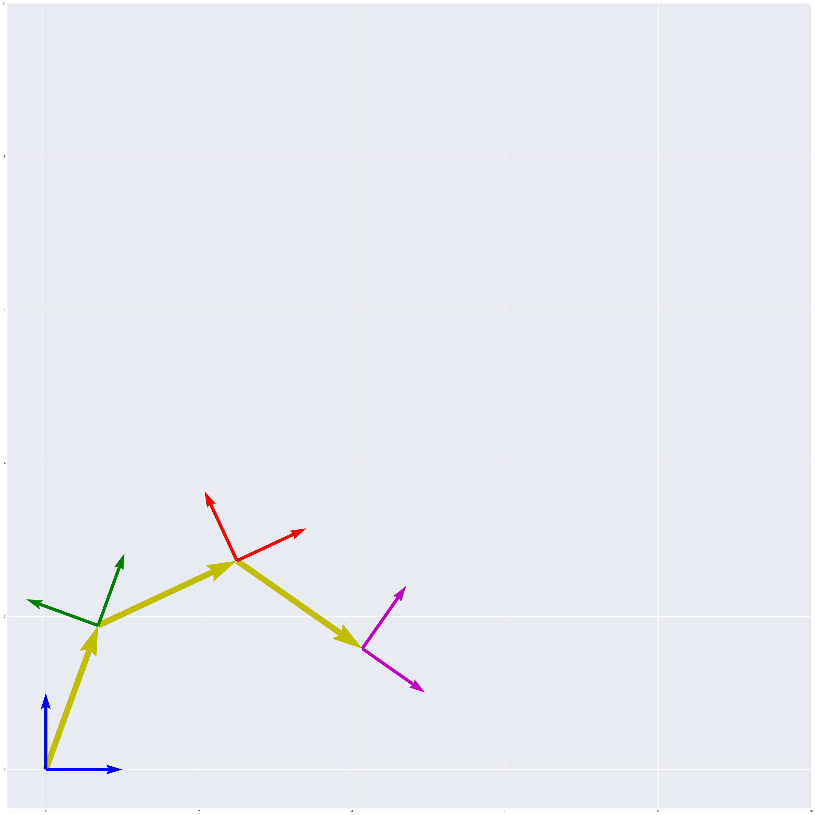
Of course, we don’t want our robot just to have one joint and one end effector, let’s try adding a second joint:
#Boilerplate
plt.gca().set_aspect('equal')        # Set aspect ratio
plt.xlim(-0.5, 3)                    # Set x-axis range
plt.ylim(-0.5, 3)                    # Set y-axis range

# frame0 defined by its origin & unit vectors
origin_0 = np.array([0, 0])
xhat_0 = np.array([1, 0])
yhat_0 = np.array([0, 1])

# Set theta0
theta0 = np.radians(30)

# Set theta1
theta1 = np.radians(30)

# Translation vector from frame0 to frame1
translation0_1 = np.array([np.cos(theta0), np.sin(theta0)])

# Translation vector from frame1 to frame2
translation1_2 = np.array([np.cos(theta0 + theta1), np.sin(theta0 + theta1)])

# Rotation matrix from frame0 to frame1
rotation0_1 = np.array([
    [np.cos(theta0), -np.sin(theta0)],
    [np.sin(theta0),  np.cos(theta0)]
])

# Rotation matrix from frame0 to frame1
rotation1_2 = np.array([
    [np.cos(theta0 + theta1), -np.sin(theta0 + theta1)],
    [np.sin(theta0 + theta1),  np.cos(theta0 + theta1)]
])

# Solve for O', x̂' and ŷ' of frame1
origin_1 = translation0_1
xhat_1 = rotation0_1.dot(xhat)
yhat_1 = rotation0_1.dot(yhat)

# Solve for O', x̂' and ŷ' of frame2
origin_2 = translation0_1 + translation1_2
xhat_2 = rotation1_2.dot(xhat)
yhat_2 = rotation1_2.dot(yhat)

# Plotting 2 unit vectors of frame0
plt.arrow(*origin_0, *xhat_0, head_width=0.05, color='b')
plt.arrow(*origin_0, *yhat_0, head_width=0.05, color='b')

# Plotting 2 unit vectors of frame1
plt.arrow(*origin_1, *xhat_1, head_width=0.05, color='g')
plt.arrow(*origin_1, *yhat_1, head_width=0.05, color='g')

# Plotting 2 unit vectors of frame2
plt.arrow(*origin_2, *xhat_2, head_width=0.05, color='r')
plt.arrow(*origin_2, *yhat_2, head_width=0.05, color='r')

# Plotting translation0_1 vector
plt.arrow(*origin_0, *translation0_1, head_width=0.05, color='y')

# Plotting translation1_2 vector
plt.arrow(*origin_1, *translation1_2, head_width=0.05, color='y')

plt.show()
![]()
Pretty neat!
Notice that we have to add transformations and thetas together is several places. This is because of the relativity. We need a way to say that frame1 is in reference to frame0, and frame2 is in reference to frame1. We do that by duplicating the math to get from frame0 to frame1 so that we can get to frame2.
There is a more concise way: homogenous transformation matrices.
Let’s take a look, and then we’ll go back and see how they work.
def coordinate_frame_plot2(plt, transformation, color='b', debug=False):
  origin = transformation.dot(np.array([0, 0, 1]))[:2]
  xhat   = transformation.dot(np.array([1, 0, 1]))[:2]
  yhat   = transformation.dot(np.array([0, 1, 1]))[:2]

  plt.arrow(*origin, *(xhat - origin), head_width=0.05, color=color)
  plt.arrow(*origin, *(yhat - origin), head_width=0.05, color=color)

  if debug:
    print("transformation_matix: ", "\n", transformation, "\n")
    print("origin: ", "\n", origin, "\n")
    print("xhat: ", "\n", xhat, "\n")
    print("yhat: ", "\n", yhat, "\n")
#Boilerplate
plt.gca().set_aspect('equal')        # Set aspect ratio
plt.xlim(-0.5, 3)                    # Set x-axis range
plt.ylim(-0.5, 3)                    # Set y-axis range

theta0 = 30
a0 = 1

theta1 = 30
a1 = 1

# Homogenous transformation from frame0 to frame0
# Identity transformation

h0 = np.array([
    [1, 0, 0],
    [0, 1, 0],
    [0, 0, 1]
])

# Homogeneous transformation from frame0 to frame1

d01 = np.array([
    [a1 * np.cos(np.radians(theta0))],
    [a1 * np.sin(np.radians(theta0))]
])

r01 = np.array([
    [np.cos(np.radians(theta0)), -np.sin(np.radians(theta0))],
    [np.sin(np.radians(theta0)),  np.cos(np.radians(theta0))]
])

h01 = np.concatenate((np.concatenate((r01, d01), 1), np.array([[0, 0, 1]])), 0)

# Homogeneous transformation from frame1 to frame2

d12 = np.array([
    [a1 * np.cos(np.radians(theta1))],
    [a1 * np.sin(np.radians(theta1))]
])

r12 = np.array([
    [np.cos(np.radians(theta1)), -np.sin(np.radians(theta1))],
    [np.sin(np.radians(theta1)),  np.cos(np.radians(theta1))]
])

h12 = np.concatenate((np.concatenate((r12, d12), 1), np.array([[0, 0, 1]])), 0)

# Plotting frames

coordinate_frame_plot2(plt, h0, color='b')
coordinate_frame_plot2(plt, h01, color='g')
coordinate_frame_plot2(plt, h01.dot(h12), color='r')
![]()